How to Run a Paired Samples T-Test in SPSS (2026): Before-and-After Data, Step by Step

If you measured the same people twice — before and after an intervention, under two conditions, at two time points — the paired samples t-test is the analysis your design calls for. It takes under a minute to run. What earns the marks is knowing why the pairing matters, checking the one assumption that actually applies, and reporting the result in the form APA 7 expects.

This walkthrough covers the whole procedure: laying out the data correctly, the assumption check, running the test, reading the output, calculating the effect size, and the fallback when the assumption fails.

Step 1: Confirm the paired test is the right one

The rule is about your design, not your variables. If each participant contributes two scores, you need the paired test. If each participant appears in only one group, you need the independent samples t-test instead.

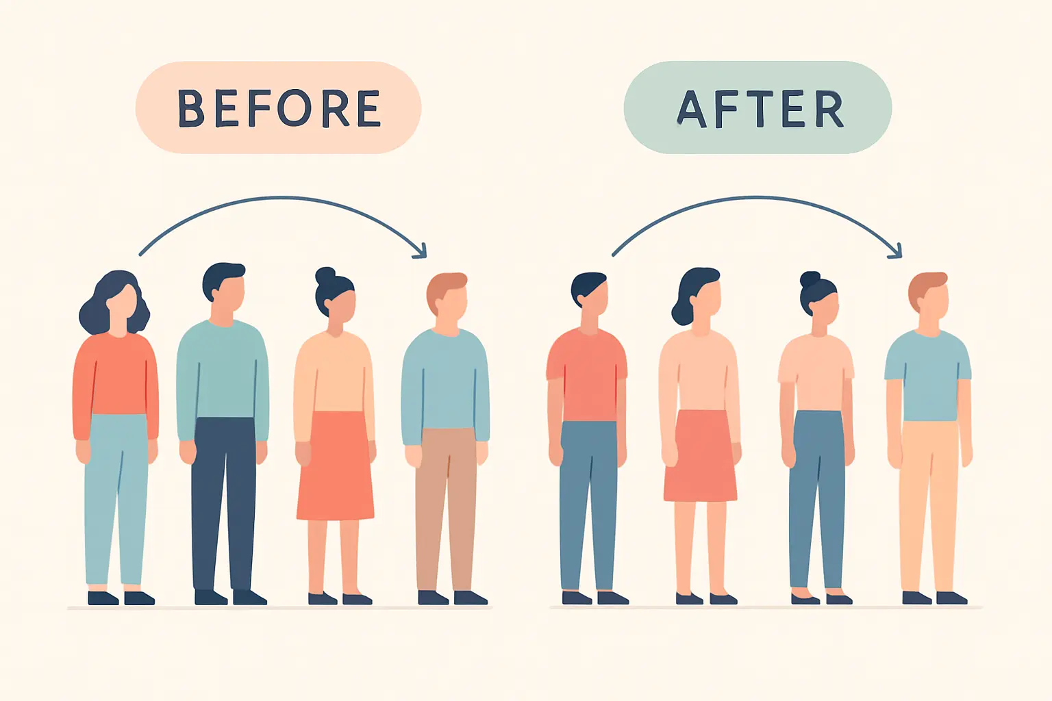
Three designs qualify as paired. A repeated measures design measures the same person before and after something. A within-subjects design measures the same person under two conditions, such as two reading formats. A matched pairs design pairs different people deliberately — twins, or participants matched on age and baseline score — and analyses them as if they were the same person measured twice.

Getting this wrong is expensive and silent. Analysing paired data with the independent test discards the pairing, which is the whole source of the design’s precision, and typically costs you the result you actually had. The reverse error, treating genuinely independent groups as paired, is simply invalid.

One further boundary: the paired t-test handles exactly two measurement occasions. With three or more you need a repeated measures ANOVA, and with three or more independent groups you need a one-way ANOVA.

Step 2: Lay the data out in wide format

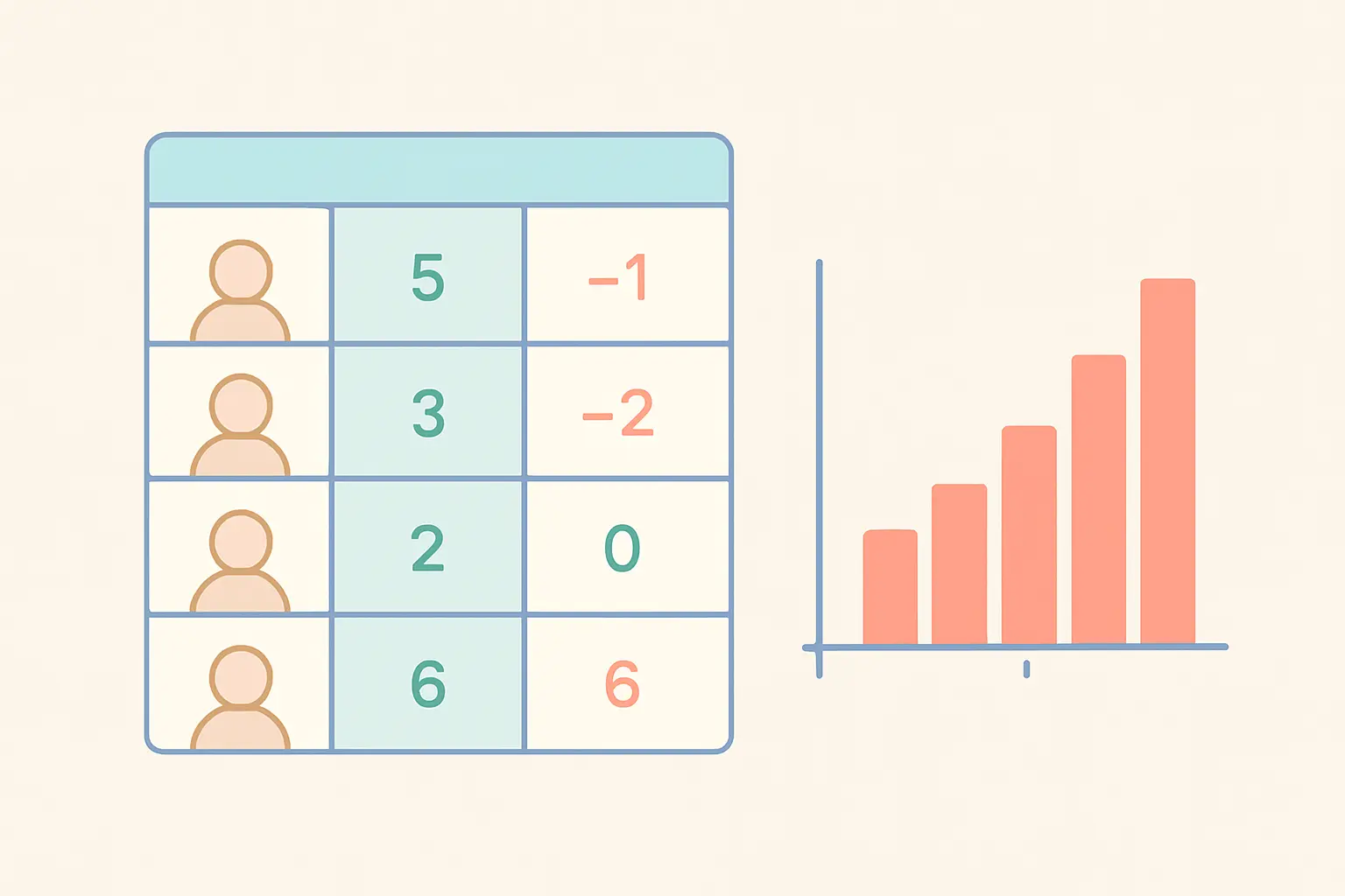
SPSS needs one row per participant with the two measurements in two separate columns — say anxiety_pre and anxiety_post. This is wide format, and it is the opposite of what many people set up by instinct.

If your data arrived in long format, with two rows per participant and a single score column, the test will not run correctly. Restructure with Data > Restructure > Restructure selected cases into variables before you go further.

Check the pairing itself before you analyse. Every row must hold the same person’s two scores, and a single misaligned row silently corrupts every difference in the file. If a participant is missing one of the two measurements, SPSS removes them from the analysis entirely — there is no partial pairing — so check your N against your expectation, and see the guide to handling missing data if the attrition is substantial.

Step 3: Check the assumption that applies

The paired test has fewer assumptions than students expect, because it is really a one-sample test performed on the difference scores.

There are three requirements. Both measurements must be continuous. The pairs must be independent of one another — your participants must not influence each other, even though each person’s own two scores are related by design. And the differences should be approximately normally distributed.

That third point is the one most often got wrong. Normality applies to the difference scores, not to the two sets of raw scores. Both measurements can be visibly skewed while their differences are perfectly symmetrical. Compute the difference as a new variable with Transform > Compute Variable, then inspect its histogram.

Do not let a significance test make this decision alone. With a large sample a normality test flags departures too trivial to affect anything; with a small one it misses departures that matter. Look at the histogram, and note that the test is fairly robust to moderate non-normality. Extreme difference scores are worth examining on their own terms — the guide to removing outliers covers what to do when one participant changed far more than everybody else.

Step 4: Run the test

Go to Analyze > Compare Means > Paired-Samples T Test.

1. Move your first measurement into Variable1 and your second into Variable2. The order sets the direction of the difference: SPSS calculates Variable1 minus Variable2, so entering the pre-test first makes an improvement show as a negative mean difference.
2. Add further pairs on the rows beneath if you have more than one, but note that each additional pair is another significance test — with several, adjust for multiple comparisons or state that the analysis is exploratory.
3. Click Options and set the confidence interval to 95 per cent. Choose how missing values are excluded.
4. Click Paste rather than OK and run the syntax from the syntax window, so you have a re-runnable record of exactly what you did.

Step 5: Read the output

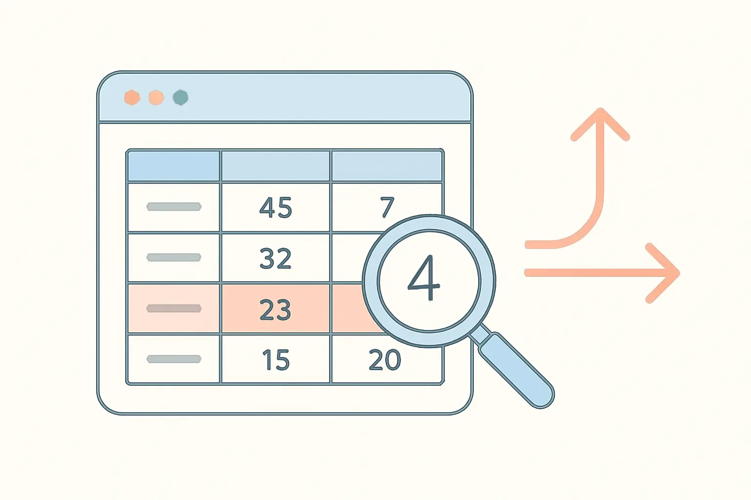
SPSS returns three tables. Paired Samples Statistics gives the mean and standard deviation of each measurement — these are your descriptives.

Paired Samples Correlations gives the correlation between the two measurements. This is not your result. It tells you how strongly the pairing holds: a high correlation means the paired design bought you real precision, which is useful to know but is not what you are testing. If it is near zero, the pairing gained you nothing, and that is worth a sentence in your discussion. The distinction between association and difference is set out in the correlation walkthrough.

Paired Samples Test is the result. Read the Mean column, which is the average difference; the 95 per cent confidence interval around it; t; df, which is the number of pairs minus one; and the significance value.

The mean difference is the number that matters, because it is expressed in your original units. A drop of 4.2 points on a 40-point anxiety scale is interpretable in a way that t = 3.71 is not. Check the sign against the order you entered the variables, and be careful never to report an improvement as a deterioration because of it.

Step 6: Calculate the effect size

Recent SPSS versions produce Cohen’s d for paired samples automatically. If yours does not, divide the mean difference by the standard deviation of the differences — both are already in your output.

The conventional benchmarks are 0.2 for a small effect, 0.5 for medium and 0.8 for large, and they should be treated as rough signposts rather than thresholds; what counts as meaningful depends on your field and on comparable published studies. Report a confidence interval around the effect size wherever you can, as the guide to effect sizes and confidence intervals explains.

One caution specific to paired designs: because the denominator is the standard deviation of the differences, paired effect sizes are typically larger than the equivalent between-groups figure and are not directly comparable with it. Say which version you calculated.

Step 7: Report it in APA 7

The conventions are specific and frequently marked. Italicise t, p, M, SD and d. Put degrees of freedom in parentheses. Give exact p-values to two or three decimals, using p < .001 only when the value is genuinely smaller. Omit the leading zero from p and d but keep it on values that can exceed 1.

A complete result reads: Anxiety scores were significantly lower after the intervention (M = 18.40, SD = 5.12) than before it (M = 22.60, SD = 5.87), t(29) = 4.31, p < .001, d = 0.79, 95% CI for the mean difference [2.21, 6.19].

That sentence contains everything a reader needs: both means, both standard deviations, the test statistic, the degrees of freedom, the exact significance, the effect size and the interval around the difference. Reporting only t and p is the most common omission.

Step 8: What to do if the assumption fails

If the difference scores are badly skewed and the sample is small, switch to the Wilcoxon signed-rank test, the rank-based equivalent that makes no distributional assumption. It is available at Analyze > Nonparametric Tests > Related Samples, and the reasoning for choosing it is set out in the guide to non-parametric tests. Report medians and interquartile ranges alongside it rather than means.

Do not run both and report whichever gives the smaller p-value. Decide on the evidence, state the decision, and give one result.

Frequently asked questions

What is the difference between a paired and an independent samples t-test?

The paired test compares two measurements from the same participants and analyses the differences within each person. The independent test compares two separate groups of people. The design decides, not the variables: if the same person appears twice in your dataset, the test is paired.

Does normality apply to my raw scores or my difference scores?

The difference scores. Both sets of raw measurements can be skewed while the differences are symmetrical, which is why you compute the difference variable and inspect that.

How many participants do I need?

Fewer than the equivalent independent design, because pairing removes between-person variability. Detecting a medium effect of d = 0.5 with 80 per cent power needs roughly 34 pairs, against about 128 participants for the independent version. Run the calculation for your own expected effect in G*Power first — see the power analysis guide.

Can I use a paired t-test on Likert data?

On a composite scale score summed or averaged across several items, yes, as it is conventionally treated as continuous. On a single Likert item, no — use the Wilcoxon signed-rank test. The item-versus-scale distinction is covered in the guide to designing a Likert scale questionnaire.

Why is my mean difference negative?

Because SPSS subtracts the second variable from the first. If you entered the pre-test first and scores rose, the difference is negative. It is not an error, but you must interpret the direction correctly in your write-up.

What does the Paired Samples Correlations table tell me?

How strongly the two measurements track each other across participants. It confirms the pairing was worthwhile but it is not your result and it does not go in your results sentence.

Can I run a paired t-test with three time points?

No. Three or more related measures require a repeated measures ANOVA. Running three paired tests instead inflates your chance of a false positive well beyond 5 per cent, and examiners look for exactly that.

What if some participants dropped out between measurements?

They are excluded from the analysis, since the test needs both scores. Report your starting N, the number of complete pairs analysed, and whether the dropouts differed systematically from those who remained — attrition that is related to the outcome is a threat to your conclusion, not just a smaller sample.

Should I report the one-tailed or two-tailed p-value?

Two-tailed, unless you predicted the direction of the change in advance and recorded that prediction. A one-tailed test chosen after seeing the direction of the result is not a legitimate halving of the p-value.

Writing up the analysis

A section that earns marks does five things in order: it names the design and why it is paired, it reports the assumption check on the difference scores, it gives both sets of descriptives, it reports the test with degrees of freedom, exact p, effect size and interval, and it interprets the mean difference in the units your reader understands.

If you are drafting that section now, Tesify can turn your SPSS output into a properly formatted APA 7 results paragraph, with the notation, the direction of the difference and the hedged interpretation already correct — leaving your time for what the change actually means.