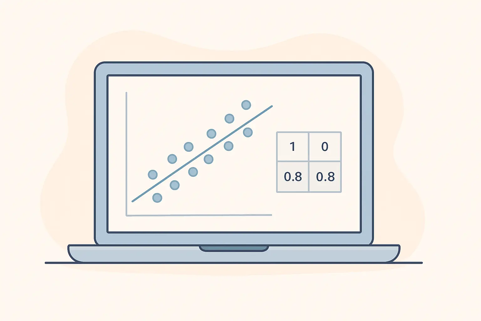
How to Run a Correlation in SPSS: Pearson, Spearman and How to Report Both (2026)

A correlation is usually the first inferential test a dissertation student ever runs, and it is the one most often reported wrongly. The analysis itself takes about forty seconds in SPSS. The decisions around it — which coefficient, which assumptions, what the number actually licenses you to claim — are what your marker reads.

This guide walks the whole procedure: choosing between Pearson and Spearman, checking the assumptions that matter, running it, reading the output, and writing it up in APA 7 format.

What a correlation actually tests

A correlation coefficient measures the strength and direction of the association between two variables. It does not test a difference between groups, and it does not identify a cause.

The coefficient runs from -1 to +1. A value of 0 means no association in the form being tested. A positive value means the two variables move together; a negative value means one rises as the other falls. The sign is a direction, not a judgement — a correlation of -.60 is exactly as strong as one of +.60.

Crucially, a correlation is symmetrical. There is no predictor and no outcome. If you need one variable to explain or predict another, you need multiple regression, not correlation. If you need to compare group means, you need ANOVA or a t-test.

Step 1: Choose Pearson or Spearman before you open SPSS

This is the decision that gets marked, and it is made from your data, not from habit.

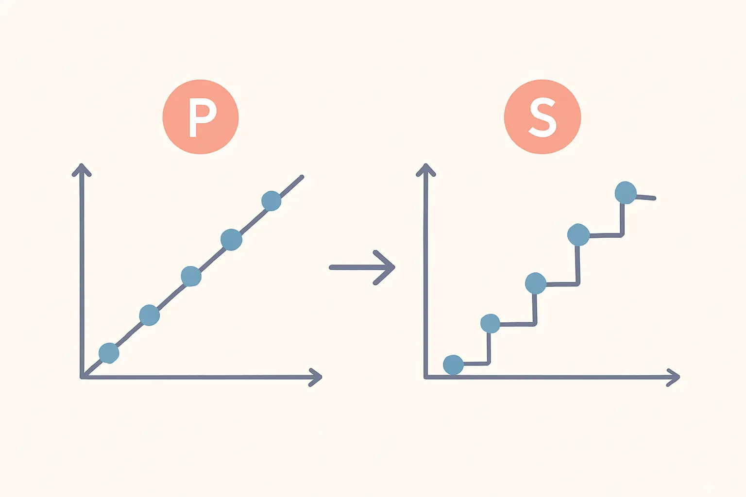
Pearson’s r tests a linear relationship between two continuous variables. Use it when both variables are interval or ratio, the relationship looks like a straight line, and there are no extreme outliers dragging the line around.

Spearman’s rho (written r_s) tests a monotonic relationship — one that consistently rises or consistently falls, but not necessarily in a straight line. It works on the ranks of your data rather than the raw values. Use it when at least one variable is ordinal, when the relationship curves but never reverses, when the data are badly skewed, or when outliers are distorting Pearson.

Kendall’s tau-b is a third option, also rank-based. It is generally preferred over Spearman when your sample is small or when many participants share the same value on a variable, because it handles tied ranks more gracefully. SPSS offers all three in the same dialog, so there is no extra work in reporting it.

A common sticking point is Likert data. A single Likert item is ordinal, so Spearman is the defensible choice. A Likert scale — several items summed or averaged into one score — is routinely treated as continuous and analysed with Pearson. If your scale is a composite, say so in your methodology and justify the treatment. Our guide to designing a Likert scale questionnaire covers the item-versus-scale distinction in full.

Step 2: Plot the scatterplot first

Never run a correlation before you have looked at the scatterplot. The coefficient is a one-number summary, and one number can hide almost anything.

In SPSS, go to Graphs > Legacy Dialogs > Scatter/Dot > Simple Scatter > Define, put one variable on each axis, and click OK.

You are looking for three things. Is the cloud of points roughly linear, or does it bend? Is the spread of points roughly even across the range, or does it fan out? Are there one or two points sitting far away from everyone else?

A curved-but-rising pattern points you to Spearman. A fanning pattern (heteroscedasticity) weakens Pearson’s significance test. A single distant outlier can turn a null result into a significant one, or the reverse — which is precisely why examiners ask to see the plot.

Step 3: Check the assumptions that apply

Pearson’s r has four practical requirements:

1. Both variables are continuous. Interval or ratio level.
2. The relationship is linear. Judged from the scatterplot in Step 2.
3. No influential outliers. Inspect the plot; if you exclude a case, report that you did and why.
4. Approximate bivariate normality. This matters for the p-value rather than for the coefficient itself, and it matters less as the sample grows.

Spearman and Kendall drop requirements 1, 2 and 4 entirely. They ask only that the relationship is monotonic and that both variables are at least ordinal. That robustness is the reason to reach for them — not a reason to reach for them by default, because on genuinely linear continuous data Pearson is the more powerful test.

Two housekeeping points before you run anything. Decide how missing values are handled — SPSS offers listwise (drop a case from every correlation if it is missing anything) or pairwise (drop it only from the pairs it affects), and pairwise deletion can leave different correlations in the same table computed on different sample sizes. Our walkthrough on handling missing data sets out when each is defensible. And check that your sample is large enough to detect the effect you are looking for; the power analysis guide covers correlation in G*Power.

Step 4: Run the correlation in SPSS

Go to Analyze > Correlate > Bivariate.

1. Move both variables into the Variables box. You can add more than two — SPSS will produce a full matrix of every pair.
2. Under Correlation Coefficients, tick Pearson, Spearman or Kendall’s tau-b as your Step 1 decision requires.
3. Under Test of Significance, leave Two-tailed selected unless your hypothesis specifies a direction in advance. A one-tailed test is only legitimate if you predicted the direction before seeing the data.
4. Tick Flag significant correlations if you want SPSS to asterisk them, though you should read the exact p-values rather than the stars.
5. Click Options to add means and standard deviations, and to set listwise or pairwise exclusion.
6. Click Paste rather than OK, and run the syntax from the syntax window. That leaves you a re-runnable record of exactly what you did.

Step 5: Read the output

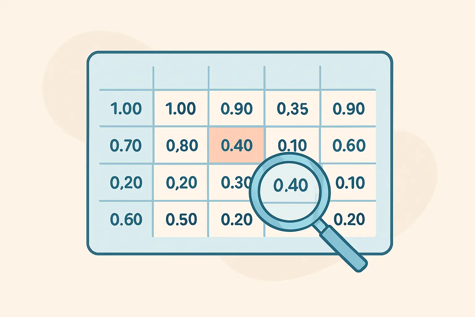
SPSS returns a square matrix. Each cell holds three rows: the coefficient, the significance value, and N.

The diagonal is always 1.000 — every variable correlates perfectly with itself — and the matrix is mirrored across it, so you only ever need to read one half. Reporting both halves is a common and easily avoided error.

For interpreting magnitude, Cohen’s conventional benchmarks are .10 for a small effect, .30 for medium and .50 for large. Treat these as rough signposts rather than thresholds: what counts as a meaningful correlation depends entirely on your field, and a coefficient of .20 can be substantively important in one literature and trivial in another. Anchor your interpretation to comparable published studies wherever you can.

Squaring the coefficient gives you the coefficient of determination. An r of .45 gives r² = .20, meaning the two variables share about 20 per cent of their variance. This is often the more honest number to put in your discussion, because it makes clear how much is left unexplained.

Note that the correlation coefficient is an effect size. You do not need to calculate a separate one, though you should report a confidence interval around it — see our guide to effect sizes and confidence intervals.

Step 6: Report it in APA 7 format

The APA 7 conventions for a correlation are specific and are frequently marked:

• Italicise r, p, N and M. Do not italicise the subscript in r_s.
• Omit the leading zero on any value that cannot exceed 1 — write .42, not 0.42. This applies to r and p.
• Report the degrees of freedom in parentheses. For a correlation, df = N – 2.
• Give exact p-values to two or three decimals. Use p < .001 only when the value is smaller than that.

A Pearson result reads: There was a moderate positive correlation between study hours and exam score, r(58) = .42, p = .001.

A Spearman result reads: Perceived workload was negatively associated with satisfaction, r_s(58) = -.38, p = .003.

If you ran more than two or three pairs, you have a multiple comparisons problem: each test carries its own chance of a false positive. Either apply a Bonferroni-style adjustment and say so, or state plainly that the analysis is exploratory and the p-values are uncorrected. Reporting fifteen pairwise correlations and celebrating the two that cleared .05 is the pattern examiners are trained to spot.

The sentence to never write

A correlation cannot establish causation, and the reason is not merely conventional caution. Three explanations always remain open: X causes Y, Y causes X, or some third variable causes both. Nothing in the coefficient distinguishes between them.

So write was associated with, was related to, predicted only in the narrow statistical sense — and never led to, caused, resulted in or improved. This single habit removes one of the most common sources of lost marks in a quantitative results chapter. For the broader picture of how correlation sits among the other designs available to you, see the quantitative research methods guide.

Frequently asked questions

Should I use Pearson or Spearman for Likert data?

Use Spearman for a single Likert item, which is ordinal. Use Pearson for a composite scale score built from several items, which is conventionally treated as continuous. State which you did and why in your methodology chapter.

What does it mean if my correlation is significant but small?

It means the association is unlikely to be zero in the population, not that it is important. Significance is heavily driven by sample size; with 500 participants an r of .09 can reach p < .05 while explaining under 1 per cent of the variance. Interpret the magnitude and the confidence interval, not the asterisk.

Can I run a correlation with a categorical variable?

Not an ordinary one. If the variable is binary you can use a point-biserial correlation, which SPSS computes as a Pearson correlation with the binary variable coded 0 and 1. For two nominal variables with more than two categories you need a chi-square test of association instead.

My Pearson and Spearman results disagree. Which do I report?

A disagreement is diagnostic: it usually means outliers or non-linearity are influencing Pearson. Go back to the scatterplot. If the relationship is monotonic but not linear, or a few extreme cases are driving the result, Spearman is the more trustworthy figure. Report it, and explain in a sentence why you chose it.

How many participants do I need for a correlation?

It depends on the effect you expect to find. Detecting a medium correlation of .30 with 80 per cent power at the conventional alpha level needs roughly 85 participants; detecting a small correlation of .10 needs several hundred. Run the calculation in G*Power before you collect data, not after.

Do I need to report a confidence interval?

APA 7 expects one wherever it is available, and it is far more informative than the p-value. A coefficient of .42 with an interval spanning .18 to .61 tells your reader how precisely you have estimated the association.

What if my data violate normality?

Normality affects the significance test rather than the coefficient. With a reasonably large sample the test is fairly robust; with a small or badly skewed sample, switch to Spearman or Kendall. The same logic that governs the choice of a non-parametric test elsewhere applies here.

Can I put correlations in a table instead of the text?

Yes, and you should once you have more than about three. An APA correlation table shows only the lower triangle, with variable names in the stub column, means and standard deviations in the final columns, and significance indicated by a note beneath the table.

Writing up the analysis

A correlation section that earns marks does four things in order: it states which coefficient was used and why, it reports the assumption checks including the scatterplot, it gives the coefficient with degrees of freedom, exact p and a confidence interval, and it interprets the magnitude against the literature rather than against Cohen’s benchmarks alone.

If you are drafting that section now, Tesify can turn your SPSS output and your notes into a properly structured results paragraph in APA 7 format, with the statistical notation and the hedged causal language already correct — so the writing time goes into interpretation rather than into formatting.