How to Run an Independent Samples T-Test in SPSS (2026): Levene’s Test, Cohen’s d and the APA Write-Up

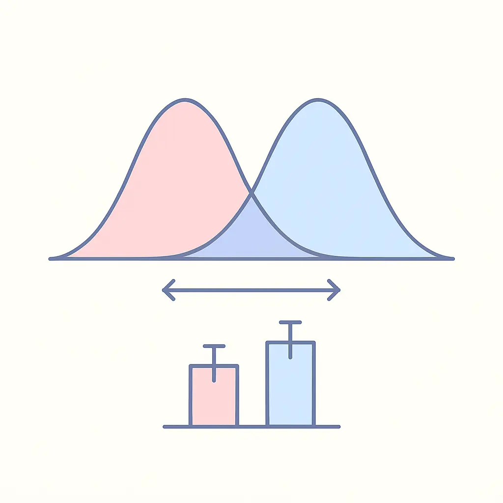
The independent samples t-test answers one question: do these two groups differ on this one measure? Men and women on a wellbeing score. Intervention and control on a post-test. Two campuses on satisfaction. It is the workhorse of the undergraduate and master’s results chapter, and the analysis takes under a minute.

What costs marks is everything around it — reading the wrong row of the output, omitting the effect size, running six t-tests where an ANOVA belonged. This guide covers the full procedure and the write-up.

Contents

• Which t-test you actually need
• The four assumptions
• Running it in SPSS
• Reading the output, including Levene’s test
• Calculating and interpreting Cohen’s d
• The APA 7 write-up, with worked examples
• What to do when an assumption fails
• Frequently asked questions

Step 1: Work out which t-test you need

SPSS offers three, and choosing the wrong one is the most consequential error in this whole procedure because it silently produces a plausible-looking number.

The independent samples t-test compares two different groups of people on one continuous measure. Each participant appears in exactly one group.

The paired samples t-test compares one group of people measured twice — before and after, or under two conditions. Each participant contributes two scores. Matched pairs count as paired too.

The one-sample t-test compares your sample mean against a known or hypothesised value, such as a published national average or a scale midpoint.

The test to reach for is dictated by the design, not by which one you have heard of. If the same person appears in both columns of your spreadsheet, you need the paired test; using the independent test there throws away the pairing and costs you statistical power.

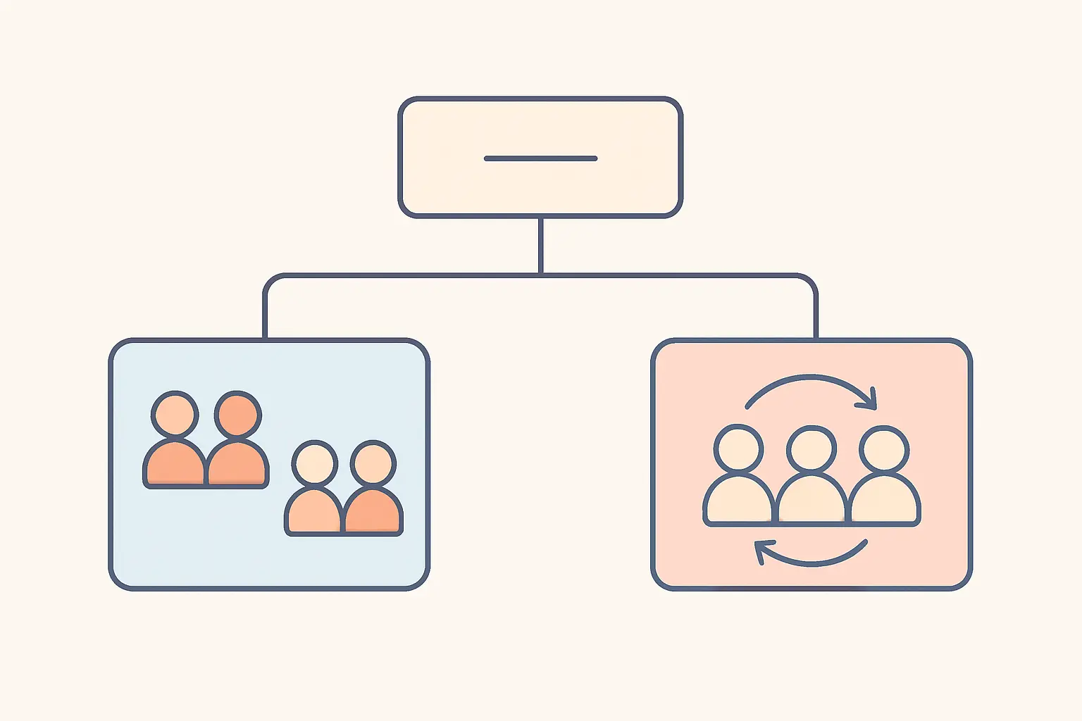
One further rule: a t-test compares exactly two groups. With three or more you need an ANOVA. Running three t-tests across three groups inflates your chance of a false positive from 5 per cent to roughly 14 per cent, and examiners look for it.

Step 2: Check the four assumptions

1. The dependent variable is continuous. Interval or ratio. A summed scale score qualifies; a single ordinal item does not.
2. Observations are independent. Each participant contributes one score, and no participant’s score influences another’s. Pupils drawn from the same three classrooms, or patients from the same handful of clinics, breach this in a way no amount of sample size repairs.
3. The dependent variable is approximately normally distributed within each group. Check with a histogram per group, or Shapiro-Wilk under Analyze > Descriptive Statistics > Explore. The t-test is fairly robust to mild departures once each group has roughly 30 or more cases.
4. Homogeneity of variance. The spread of scores should be similar in the two groups. SPSS tests this for you with Levene’s test, inside the same output table — so you do not need to run it separately.

Before collecting data, check the design can detect the effect you are chasing. Detecting a medium standardised difference of 0.5 with 80 per cent power needs about 64 participants per group; a small difference of 0.2 needs close to 400 per group. The G*Power walkthrough covers the calculation.

Step 3: Run it in SPSS

Your data need two columns: one continuous outcome variable, and one grouping variable coded with two values (for example 1 = control, 2 = intervention). One row per participant.

1. Go to Analyze > Compare Means > Independent-Samples T Test.
2. Move your continuous outcome into the Test Variable(s) box.
3. Move your two-group variable into the Grouping Variable box.
4. Click Define Groups and enter the two codes — 1 and 2 in the example above. SPSS will not run until you do this, and the question marks beside the variable name are the reminder.
5. Under Options, confirm the confidence interval is set to 95 per cent and choose how missing values are excluded.
6. Click Paste instead of OK and run from the syntax window, so you keep a re-runnable record of the analysis.

Step 4: Read the output — and start with Levene’s test

SPSS returns two tables. Group Statistics gives you N, mean and standard deviation for each group; those numbers go straight into your write-up. Independent Samples Test holds the result.

That second table has two rows, and you report exactly one of them. Which one is decided by Levene’s test in the leftmost columns.

• Levene’s p is greater than .05 — variances are comparable. Read the top row, “Equal variances assumed”.
• Levene’s p is .05 or below — variances differ. Read the bottom row, “Equal variances not assumed”. This is the Welch correction, and you will notice its degrees of freedom are not a whole number.

Note the logic runs opposite to your instincts elsewhere: here a significant Levene’s test is the inconvenient result. It is not a reason to abandon the analysis. The Welch row is a perfectly respectable test — many statisticians argue it should simply be the default — so you report it and move on.

From your chosen row, take four things: t, df, the two-sided p value (labelled “Sig. (2-tailed)” in older SPSS versions and “Two-Sided p” in recent ones), and the 95% Confidence Interval of the Difference. That interval is the most useful number in the table and the one students most often skip.

Step 5: Get the effect size

A p-value tells you whether a difference is detectable. It does not tell you whether it matters. APA 7 requires an effect size alongside it, and for a t-test that means Cohen’s d.

Recent SPSS versions produce it automatically in an “Independent Samples Effect Sizes” table. In older versions, calculate it by dividing the mean difference by the pooled standard deviation.

Cohen’s conventional benchmarks are 0.2 for a small effect, 0.5 for medium and 0.8 for large — signposts rather than thresholds, and worth less than a comparison against effect sizes reported in your own literature. A d of 0.3 may be a meaningful clinical gain in one field and noise in another. Our guide to effect sizes and confidence intervals covers interpretation and reporting in more depth.

Step 6: Write it up in APA 7

The APA formatting rules that get marked here are consistent: italicise t, p, d, M, SD and n; omit the leading zero on p because it cannot exceed 1, but keep it on t, M, SD and d, which can; give exact p-values to two or three decimals, reserving p < .001 for values genuinely smaller than that.

Equal variances assumed:

An independent samples t-test found that intervention participants (M = 24.60, SD = 4.12, n = 30) scored significantly higher than control participants (M = 21.83, SD = 4.05, n = 30), t(58) = 2.63, p = .011, d = 0.68, 95% CI [0.66, 4.88].

Equal variances not assumed:

Levene’s test indicated unequal variances, F = 6.21, p = .016, so the Welch correction was applied. The difference remained significant, t(48.37) = 2.41, p = .020, d = 0.62.

Notice three habits in those sentences. Both group means and standard deviations appear, so the reader can see the size of the difference in the original units. The unequal-variance case says so explicitly rather than leaving the reader to wonder why df has decimals. And the confidence interval is present.

What to do when an assumption fails

Unequal variances. Nothing to do — read the Welch row and say you did.

Non-normal data. With reasonably sized groups the t-test tolerates moderate skew. With small or severely skewed groups, switch to the Mann-Whitney U test, the rank-based equivalent. Report the median and interquartile range rather than the mean, and explain the switch in a sentence.

Non-independent observations. This one is not fixable within a t-test. If participants are clustered inside schools, wards or teams, the analysis needs to model that structure. Do not simply proceed and hope.

An ordinal outcome. A single Likert item is ordinal; use Mann-Whitney. A multi-item scale score is conventionally treated as continuous and is fine.

Frequently asked questions

What if Levene’s test is significant?

Read the second row of the output, “Equal variances not assumed”. The analysis is still valid — SPSS has applied the Welch correction, which adjusts the degrees of freedom to compensate. State in your write-up that variances were unequal and the correction was used.

Can I use a t-test with different sample sizes in each group?

Yes. Unequal group sizes are fine and very common. They do make the test more sensitive to unequal variances, which is one more reason to read Levene’s test carefully rather than defaulting to the top row.

Why are my degrees of freedom not a whole number?

Because you are reading the Welch row. The correction adjusts df downwards to a fractional value. Report it as SPSS gives it, rounded to two decimals — t(48.37), not t(48).

Should I use a one-tailed or two-tailed test?

Two-tailed, unless you stated a directional hypothesis before you saw any data. Switching to one-tailed after the fact to push a p-value under .05 is a recognised questionable research practice, and the halved p-value is not defensible in a viva.

My result is not significant. Have I failed?

No. A non-significant t-test is a finding, and it is reported the same way, with the effect size and the confidence interval. A wide interval spanning zero tells your reader the study could not settle the question, which is a different and more honest claim than saying there is no difference.

Do I need to report Cohen’s d if the result is non-significant?

Yes. The effect size describes the magnitude of the difference you observed regardless of whether it cleared the significance threshold, and it is what future meta-analyses will use.

Can I run several t-tests instead of one ANOVA?

Not for three or more groups. Each additional test carries its own false-positive risk, and the errors compound. Use an ANOVA with an appropriate post-hoc correction. Multiple t-tests across a set of groups is one of the most reliably penalised patterns in a quantitative results chapter.

How is this different from a correlation?

A t-test compares two group means on one measure; a correlation measures how two continuous variables move together across a single sample. Different questions, different data structures. If you want to predict one variable from several others, you want regression instead.

Bringing it together

A results paragraph that earns marks names the test and why it was chosen, reports the assumption checks including Levene’s outcome, gives the group descriptives, states t with its degrees of freedom and an exact p-value, adds Cohen’s d and the confidence interval, and then interprets the size of the difference against the literature rather than against Cohen’s labels alone.

The statistics are the quick part. If the write-up is what is holding you up, Tesify will take your SPSS output and turn it into a structured APA 7 results section with the notation, the italics and the hedging already correct — leaving you to spend your time on what the difference actually means. For the wider context of where the t-test sits among your options, the quantitative research methods guide maps the whole territory.