
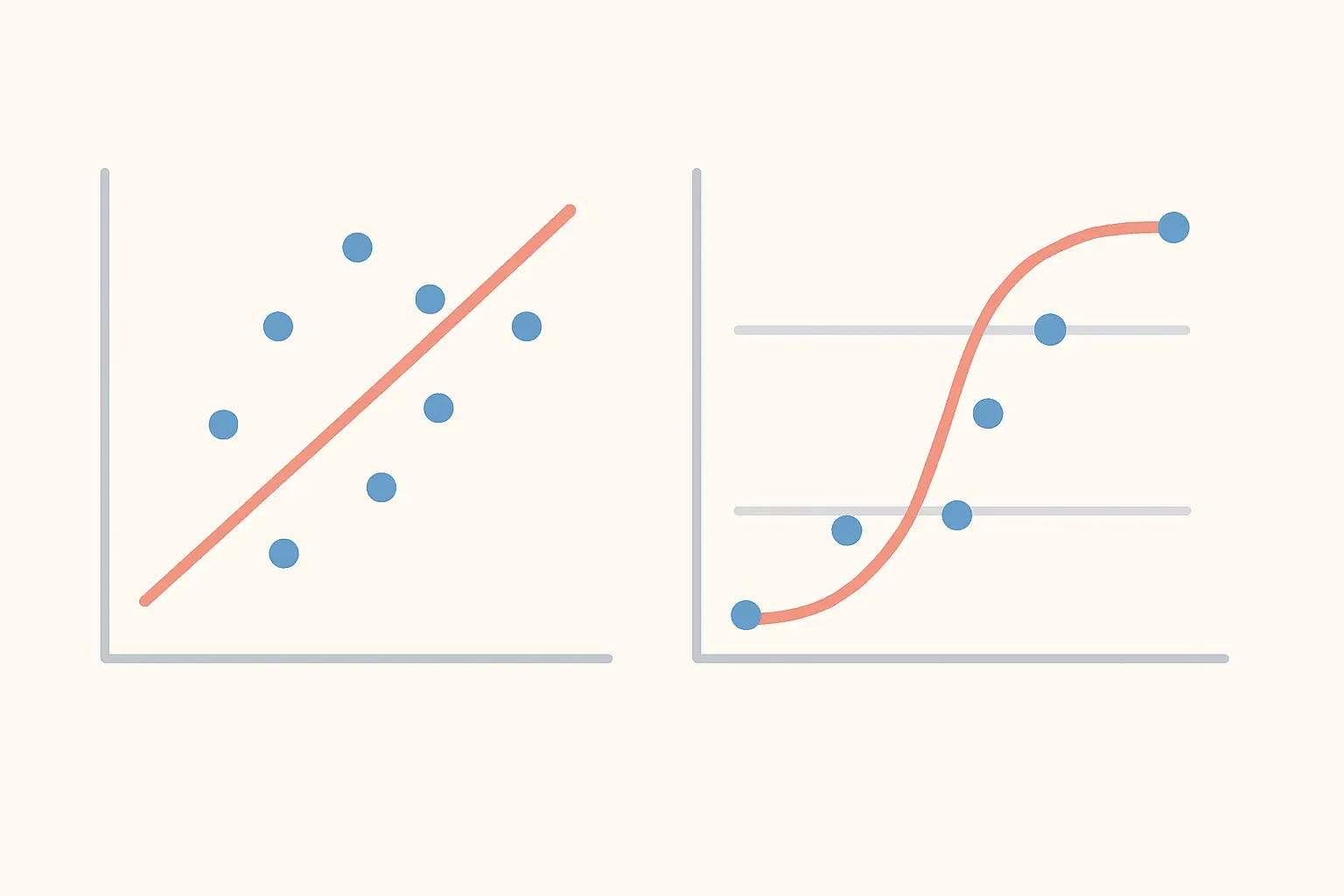
Linear vs Logistic Regression (2026): Which One Does Your Outcome Variable Need?
Students almost never choose the wrong regression on purpose. They choose it because linear regression is the one they were taught, and their outcome variable happens to be coded 0 and 1 — so SPSS runs it, produces coefficients, and says nothing. The output looks entirely normal. It is wrong.
The rule is short: the type of your outcome variable decides the model. Everything else follows from that.
The comparison at a glance
| Linear regression | Binary logistic regression | |
|---|---|---|
| Outcome variable | Continuous (score, income, time, temperature) | Binary — two categories (passed/failed, churned/stayed, diagnosed/not) |
| What it predicts | A value on the outcome’s own scale | The probability of the outcome occurring |
| Shape of the fit | A straight line | An S-shaped curve, bounded by 0 and 1 |
| Coefficient meaning | B = change in Y per one-unit rise in X | B = change in the log-odds; Exp(B) = odds ratio |
| Headline fit statistic | R² | Nagelkerke R² (a pseudo-R²) plus the classification table |
| Significance of a predictor | t-test on the coefficient | Wald chi-square test |
| Needs normal residuals? | Yes | No |
| Needs equal variance of residuals? | Yes | No |
| SPSS menu path | Analyze > Regression > Linear | Analyze > Regression > Binary Logistic |
Why you cannot simply run linear regression on a 0/1 outcome
Three things break, and each one is visible to a marker who knows where to look.
The predictions escape the possible range. A straight line has no ceiling and no floor. Fit one to a binary outcome and it will happily predict a probability of 1.3 for some participants and -0.2 for others. Those are not unlikely values; they are impossible ones.
The residuals cannot be normal. When the observed value is only ever 0 or 1, every residual is one of exactly two numbers for any given prediction. Normality of residuals is not merely violated here — it cannot hold even in principle.
The variance is structurally unequal. For a binary outcome the variance depends on the probability itself, and is largest near 0.5 and smallest at the extremes. Homoscedasticity fails by construction, which distorts the standard errors and therefore every p-value in the table.
One honest caveat, because your supervisor may raise it: economists do sometimes fit a “linear probability model” to binary data deliberately, using robust standard errors, because the coefficients are easy to interpret as changes in probability. That is a considered choice within a specific tradition, defended in the write-up. It is not the same thing as running linear regression on a binary outcome without noticing.
Start from your outcome variable

- Continuous — exam mark, salary, blood pressure, minutes taken. Use linear regression.
- Binary — two categories only. Use binary logistic regression.
- Ordinal — three or more ordered categories, such as low/medium/high satisfaction. Use ordinal logistic regression, which adds a proportional odds assumption you must test.
- Nominal with three or more unordered categories — such as which of four transport modes someone chose. Use multinomial logistic regression.
- Counts — number of absences, number of citations. Use Poisson or negative binomial regression, not either of the two models compared here.
A related trap is worth naming. If your outcome is genuinely continuous, resist the urge to split it at the median to “make it binary” so you can run logistic regression. Dichotomising a continuous variable throws away real information, reduces statistical power, and is treated as a methodological weakness rather than a simplification.
Running binary logistic regression in SPSS
- Code your outcome so that the event of interest is 1 and its absence is 0. Getting this backwards inverts every odds ratio you report.
- Go to Analyze > Regression > Binary Logistic.
- Move your binary outcome into Dependent and your predictors into Covariates.
- Click Categorical and declare any categorical predictors, choosing a sensible reference category. Every odds ratio is relative to that reference, so choosing it carelessly makes your results hard to read.
- Under Options, tick Hosmer-Lemeshow goodness-of-fit and CI for exp(B). The confidence interval is required for the write-up.
- Click Paste and run from the syntax window so the analysis is reproducible.
What logistic regression still assumes
Dropping normality and homoscedasticity does not make the model assumption-free:
- Independent observations. Same requirement as everywhere else.
- Linearity of the logit for any continuous predictor — the relationship must be linear on the log-odds scale, testable with the Box-Tidwell procedure.
- No serious multicollinearity among predictors, checked the same way as in linear regression.
- Enough events per predictor. The working guideline is at least ten cases in the smaller outcome category for every predictor you enter. With 40 events you are stretching four predictors, whatever your total sample size.
- No complete separation. If a predictor perfectly divides the two outcomes, SPSS will return enormous coefficients with enormous standard errors. That is a warning sign, not a strong finding.
On sample size, note that the constraint is the number of events, not the number of participants. A study of 500 people containing only 25 cases of the outcome is a small study for these purposes. The power analysis guide covers planning this properly.
Reading the output
Omnibus Tests of Model Coefficients asks whether your model beats a model with no predictors at all. A significant chi-square here is the equivalent of a significant F-test in linear regression.
Model Summary reports Cox & Snell R² and Nagelkerke R². These are pseudo-R² measures. They do not mean “percentage of variance explained” and should not be described as such — report Nagelkerke, and describe it as an approximate indication of model strength.
Hosmer-Lemeshow inverts the usual logic: a non-significant result indicates acceptable fit. The test is sensitive to sample size and is increasingly criticised, so treat it as one signal among several rather than a verdict.
The Classification Table shows how many cases the model sorts correctly. Read it against the base rate: if 85 per cent of your sample did not experience the outcome, a model that predicts “no” for everybody is already 85 per cent accurate and has learned nothing.
Variables in the Equation is the table you report. It gives B, the standard error, the Wald statistic, the p-value, and Exp(B) — the odds ratio — with its confidence interval.

Interpreting the odds ratio without overclaiming
Exp(B) is the multiplicative change in the odds of the outcome for a one-unit increase in the predictor. Above 1 the odds increase; below 1 they decrease; at 1 there is no effect. So an Exp(B) of 1.45 means a one-unit rise in the predictor multiplies the odds of the outcome by roughly 1.45 — a 45 per cent increase in the odds.
Two cautions. First, the confidence interval decides significance more reliably than the p-value does: if the interval for Exp(B) contains 1, the effect is not statistically significant, regardless of what the coefficient looks like.
Second — and this is the interpretive error markers look for — odds are not probability, and an odds ratio is not a risk ratio. When the outcome is rare the two are close. When the outcome is common the odds ratio substantially overstates the change in risk. An odds ratio of 2.0 on an outcome that already occurs in 40 per cent of cases does not mean the outcome becomes twice as likely.
Because of that, avoid writing “twice as likely” for an odds ratio of 2. Write “the odds were twice as high” instead. The precision costs you nothing and protects the claim.
Reporting it in APA 7
A binary logistic regression was conducted to predict placement completion from age, prior experience and study mode. The model was significant, χ²(3) = 24.17, p < .001, and explained approximately 18 per cent of the variation in the outcome (Nagelkerke R² = .18), correctly classifying 74.2 per cent of cases. Prior experience was a significant predictor, B = 0.62, SE = 0.21, Wald χ²(1) = 8.71, p = .003, OR = 1.86, 95% CI [1.23, 2.81].
Report the odds ratio and its confidence interval for every predictor, not only the significant ones, and state which category was the reference for each categorical predictor.
Frequently asked questions
Can I use linear regression if my binary outcome is roughly 50/50?
A balanced outcome makes the impossible-prediction problem less visible, but it does not fix the non-normal residuals or the structural heteroscedasticity. Use logistic regression, and if you have a specific reason to prefer a linear probability model, say so and use robust standard errors.
What is a good Nagelkerke R-squared?
There is no threshold, and values look low compared with linear regression R² even for useful models. Judge it against comparable published studies in your field rather than against any absolute standard, and lean on the classification table and the individual odds ratios instead.
What if one of my predictors perfectly predicts the outcome?
That is complete separation. SPSS will produce a huge coefficient with a huge standard error and a non-significant p-value, which is the model failing rather than an unusually strong finding. Usually it means a category is too small or a predictor overlaps the outcome definition. Collapse categories or remove the predictor, and say why.
How do I compare two logistic models?
Enter the predictors in blocks and compare the -2 log likelihood values. SPSS reports the change as a chi-square with degrees of freedom equal to the number of added predictors, which tests whether the extra variables improved the model.
Is logistic regression the same as a chi-square test?
No, though they answer related questions. A chi-square test examines association between two categorical variables on their own. Logistic regression estimates the effect of each predictor while holding the others constant, and handles continuous predictors.
Can I include both continuous and categorical predictors?
Yes, and that is the usual case. Declare the categorical ones in the Categorical dialog and set the reference category deliberately — the odds ratios are meaningless if you do not know what they are being compared against.
Which do I use to compare two groups on a continuous outcome?
Neither, if that is your only question — an independent samples t-test answers it directly. And if you want to know how two continuous variables move together without predicting one from the other, you want a correlation.
The recommendation
There is no contest between these two models, because they are not competitors. Read your outcome variable, and let it choose. Continuous outcome, linear regression. Binary outcome, logistic regression. Ordered categories, ordinal logistic. Counts, Poisson.
The one decision that genuinely costs marks is defaulting to linear regression because it is the familiar one and then never checking whether the outcome could support it. Thirty seconds spent identifying the measurement level of your dependent variable prevents a chapter’s worth of invalid results. For a broader map of how these models sit alongside the rest of your options, see the quantitative research methods guide, and for reporting conventions the guide to effect sizes and confidence intervals.
Once the model is chosen and run, Tesify can turn the SPSS output into a properly formatted APA 7 results section — with the odds ratios, the confidence intervals and the carefully hedged interpretation already in the right shape.
Write your thesis with AI
Structure, draft, cite, and format your thesis faster with Tesify’s AI writing tools, automatic bibliography, and plagiarism checker. Free to start, no credit card required.






Leave a Reply