How to Run PLS-SEM in SmartPLS (2026): Measurement Model, Bootstrapping and What to Report

PLS-SEM has become the default analysis for master’s and doctoral theses in business, management, information systems and marketing — partly because it handles the small samples and complex models those fields produce, and partly because SmartPLS makes it clickable. That accessibility is also the problem: the software will happily produce a beautiful path diagram from data that fails every quality criterion, and it will not tell you. This guide covers the full sequence, in the order the assessment has to happen, and the specific numbers examiners expect to see.

First: is PLS-SEM actually the right choice?

PLS-SEM is a variance-based method. It estimates composite constructs to maximise explained variance in your dependent variables, which makes it prediction-oriented. Covariance-based SEM instead tries to reproduce the observed covariance matrix, which makes it confirmation-oriented and gives you global fit statistics. They answer different questions, and the choice is a methodological argument you must make in writing.

PLS-SEM is the defensible choice when your goal is prediction or explaining variance in a target construct, when your model is complex with many constructs and indicators, when you have formatively measured constructs, when your sample is modest, or when the data are badly non-normal. Covariance-based SEM is the better choice when you are testing a well-established theory and want global fit indices, and our guide to structural equation modelling, path models, CFA and fit indices covers that route in full.

One warning about sample size. The old “ten times rule” — ten cases per the largest number of arrows pointing at any construct — is still widely quoted and is no longer considered adequate on its own. Justify your sample with a formal power analysis for the most complex regression in your model, or with the inverse square root method, rather than citing the rule of thumb. Our sample size and power analysis guide walks through the calculation.

Step 1: Specify the model, and get reflective vs formative right

This single decision determines every quality criterion you will apply later, and getting it wrong invalidates the whole assessment. It is also the mistake reviewers catch most often.

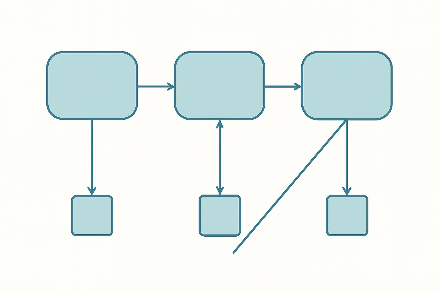
In a reflective measurement model the construct causes the indicators. Arrows point outward from the construct. The items are interchangeable manifestations of the same underlying thing, so they should correlate highly, and dropping one should not change what the construct means. Most attitude and perception scales are reflective.

In a formative measurement model the indicators cause the construct. Arrows point inward. The items are not interchangeable — each captures a distinct facet — so they need not correlate, and dropping one genuinely changes the construct’s meaning. A socioeconomic status index built from income, education and occupation is formative.

The test is a thought experiment: if a respondent’s score on the construct rose, would every indicator rise with it? If yes, reflective. If the indicators are separate components that together compose the construct, formative. Decide this from theory before you touch the software, and state it in your methodology.

Step 2: Prepare and import the data

SmartPLS reads CSV and Excel files with one row per case and one column per indicator. Before importing, deal with the practical issues that will otherwise surface as confusing errors.

Give every column a short name without spaces, mapping to your questionnaire item. Reverse-score negatively worded items before import — PLS will not do it for you, and an unreversed item shows up later as a negative loading you might mistake for a substantive finding. Code missing values consistently with a single marker such as -99 and declare it on import; if more than about 5% of values on any indicator are missing, address that rather than letting mean replacement quietly paper over it. Finally, screen for straight-lining and impossibly fast completions, and document how many cases you removed and why.

Then draw the model on the canvas: create each latent variable, assign its indicators, and connect the constructs with the paths your hypotheses specify. Set each construct’s measurement mode to reflective or formative to match Step 1.

Step 3: Run the PLS algorithm

Use the default settings unless you have a reason not to: path weighting scheme, standardised data, maximum 300 iterations, stop criterion 10^-7. Two things to check immediately.

Did the algorithm converge? If it ran to the maximum iterations without converging, something is wrong with the model or the data — usually a construct with too few indicators, or near-perfect collinearity.

Are any loadings negative? A negative loading on a reflective construct almost always means an unreversed item, not a discovery.

The PLS algorithm gives you point estimates only. It produces no p-values and no confidence intervals — those come from bootstrapping in Step 6. Do not report a path as significant on the basis of this run.

Step 4: Assess the reflective measurement model

Four criteria, in order. Every one has a conventional threshold, and every threshold is a guideline you may depart from with justification, not a law.

Indicator reliability. Outer loadings should be at least 0.708, which means the construct explains more than half the indicator’s variance. Items loading between 0.40 and 0.708 are a judgement call: remove one only if doing so raises composite reliability or AVE above its threshold, and never remove an item purely to improve a number if it costs you content validity. Loadings below 0.40 should generally go.

Internal consistency reliability. SmartPLS reports Cronbach’s alpha, composite reliability (ρ_c) and ρ_A. Alpha assumes all indicators are equally weighted and tends to understate reliability; composite reliability tends to overstate it; ρ_A usually sits between them and is a reasonable compromise. Values from 0.70 to 0.90 are satisfactory. Values above 0.95 are a problem, not a triumph — they suggest your items are near-redundant restatements of each other. For the wider reliability picture, see our guide to Cronbach’s alpha and how to report reliability.

Convergent validity. Average variance extracted should be 0.50 or above, meaning the construct explains at least half the variance of its indicators on average.

Discriminant validity. The current standard is the heterotrait-monotrait ratio (HTMT). The conservative threshold is 0.85; 0.90 is acceptable for constructs that are conceptually similar. The older Fornell-Larcker criterion and cross-loadings are still commonly reported alongside it, but HTMT is substantially better at detecting a discriminant validity problem and should lead. If HTMT exceeds the threshold, your two constructs are not empirically distinct — merge them, drop one, or respecify. Bootstrapping also lets you test whether HTMT is significantly below 1, which is the stronger test.

Step 5: Formative constructs are assessed completely differently

None of Step 4 applies to a formative construct. Internal consistency is meaningless when indicators are not expected to correlate, and reporting Cronbach’s alpha for a formative construct is a clear signal to an examiner that the distinction was not understood. Three different criteria apply.

Convergent validity via redundancy analysis. Model the formative construct as a predictor of a reflective or single-item measure of the same concept; the path should be at least 0.70. This requires you to have included that global item in your questionnaire, which is why the reflective/formative decision has to happen before data collection.

Indicator collinearity. Check VIF for the formative indicators. Values below 3 are ideal; values at or above 5 indicate a collinearity problem that makes the individual weights uninterpretable.

Significance and relevance of outer weights. Bootstrap the outer weights. If a weight is non-significant but its loading is 0.50 or above, the indicator can usually be retained on theoretical grounds; if both are low, consider removing it — but remember that removing a formative indicator removes part of the construct itself.

Step 6: Bootstrap for significance

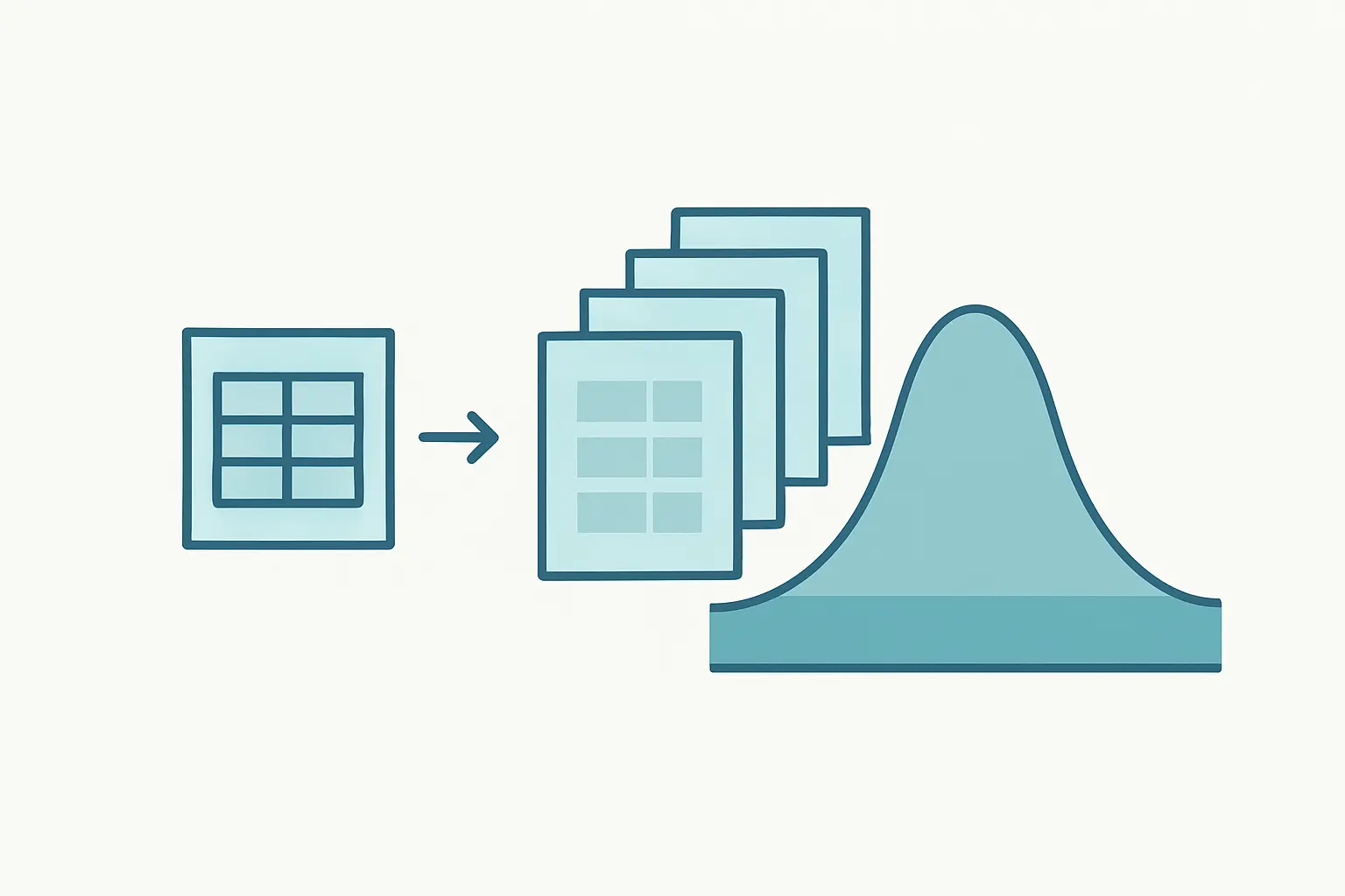
PLS-SEM makes no distributional assumptions, so significance comes from resampling rather than from a theoretical distribution. Bootstrapping draws thousands of samples with replacement from your data, re-estimates the model in each, and builds an empirical distribution for every parameter.

Use 10,000 subsamples for your final reported results — 5,000 is the older convention and is still widely accepted, but more subsamples give more stable estimates and the run is cheap. Use a smaller number only while exploring. Report bias-corrected and accelerated confidence intervals where available; percentile intervals are an acceptable alternative.

Two points that matter for interpretation. First, report confidence intervals, not just p-values — an interval that excludes zero is the cleaner statement, and it shows the precision of the estimate rather than only its significance. Second, use one-tailed tests only if your hypothesis is genuinely directional and you said so in advance; two-tailed is the safer default.

Bootstrap results vary slightly between runs because the resampling is random. This is expected. Do not re-run until you get a p-value you like — that is p-hacking with extra steps.

Step 7: Assess the structural model

Only once the measurement model passes do you interpret the paths. Assessing structural relationships between constructs you have not established as reliable and valid is meaningless.

Collinearity between predictors. Inner VIF values should be below 3. Higher values mean your predictor constructs overlap enough to destabilise the path estimates.

Path coefficients. Standardised, running roughly from -1 to +1. Report the coefficient, the confidence interval and the p-value for each hypothesis, and say plainly whether it is supported.

R². Variance explained in each endogenous construct. The often-cited benchmarks of 0.25, 0.50 and 0.75 for weak, moderate and substantial are discipline-dependent — in consumer behaviour 0.20 can be high, while a model predicting a closely related outcome might need far more. Interpret against comparable published work in your field, not against the generic benchmark.

f² effect size. The change in R² when a predictor is removed: 0.02, 0.15 and 0.35 indicate small, medium and large effects. This is what tells you whether a statistically significant path is actually consequential.

Q² predictive relevance. Obtained by blindfolding; a value above zero means the model has predictive relevance for that construct. For genuine out-of-sample prediction, run PLSpredict and compare the PLS-SEM prediction errors against the linear model benchmark.

A note on model fit. SmartPLS reports SRMR, with 0.08 commonly cited as a threshold. Global fit measures are contested in a PLS-SEM context because the method does not optimise for fit, so treat SRMR as supplementary evidence rather than a pass/fail gate, and do not build your case on it.

Step 8: Mediation and moderation

For mediation, use the bootstrapped indirect effect rather than the old causal-steps procedure. Test the indirect effect first: if it is significant, examine the direct effect to characterise the mediation as complementary partial, competitive partial, or full. If the indirect effect is not significant, there is no mediation to describe, whatever the direct effect does.

For moderation, create the interaction term using the two-stage approach, which handles formative constructs and is the general-purpose default. Report the interaction path and a simple slope plot; the interaction effect size is typically small, and f² around 0.005 can still be meaningful for interactions.

What to report in your thesis

A complete PLS-SEM results section runs in a fixed order, and examiners look for the sequence as much as the numbers.

State the software and version, the algorithm settings and the number of bootstrap subsamples. Justify PLS-SEM over covariance-based SEM explicitly. Report the measurement model first — a table of loadings, alpha, ρ_A, composite reliability and AVE per construct, then an HTMT matrix — and state which items were removed and why. Report formative constructs separately with VIF and outer weights. Only then present the structural model: inner VIF, then a table of path coefficients with confidence intervals and p-values against each hypothesis, then R², f² and Q². Include the path diagram.

PLS-SEM is standard in technology acceptance research, so if your model extends TAM or UTAUT, our comparison of TAM and UTAUT for dissertations covers the model choice that sits upstream of this analysis. If you are still choosing software, our comparison of data analysis software for theses sets out the alternatives.

Frequently asked questions

What sample size do I need for PLS-SEM?

There is no single number. The ten times rule is no longer considered adequate justification on its own. Run a power analysis for the most complex regression in your model — the endogenous construct with the most predictors — or use the inverse square root method, and report the calculation.

Can I use PLS-SEM with a small sample?

It tolerates smaller samples better than covariance-based SEM, but “PLS works with small samples” is not a justification for an underpowered study. Small samples produce wide confidence intervals and unstable estimates regardless of method.

Should I report Cronbach’s alpha or composite reliability?

Report both, plus ρ_A. Alpha is a lower bound and composite reliability an upper bound, so reporting all three shows the range rather than letting you pick the flattering one. Report none of them for formative constructs.

What is the difference between HTMT and the Fornell-Larcker criterion?

Both assess discriminant validity, but Fornell-Larcker performs poorly at detecting problems when indicator loadings differ little. HTMT is more sensitive and should be your primary criterion; report Fornell-Larcker alongside it if your field expects it.

How many bootstrap subsamples should I use?

10,000 for final results. 5,000 remains widely accepted, and smaller numbers are fine while you are still exploring the model.

My model fit (SRMR) is above 0.08 — is that fatal?

Not necessarily. Global fit indices are contested in PLS-SEM because the method does not minimise a fit function. Discuss it honestly, but rest your evaluation on the measurement and structural criteria rather than on SRMR.

Can I remove indicators to improve my numbers?

Only within limits, and only with justification. Dropping a reflective item with a low loading is defensible if it lifts AVE or reliability past the threshold and the construct’s content is preserved. Dropping items until everything passes is specification searching, and you must report every removal.

Is PLS-SEM criticised in the literature?

Yes, and you should acknowledge it. There is a substantial methodological debate about PLS-SEM’s status as a latent-variable technique and about its statistical properties. Cite the criticism, explain why the method still fits your objective, and you convert a vulnerability into evidence of methodological awareness.

Turn the analysis into a methodology chapter

A PLS-SEM results chapter is a long, ordered sequence of tables and justifications, and most of it has to be written while you still remember which items you dropped and why. Tesify helps you build the methodology and results chapters around your own analysis decisions as you make them, so the reporting sequence is complete before the deadline — 100% written by you.

Write your thesis with Tesify