
Structural Equation Modeling (SEM) Explained 2026: Path Models, CFA, and Fit Indices
Your committee has asked why you chose structural equation modeling over multiple regression, and you need an answer that goes beyond “the literature used it.” Structural equation modeling is a multivariate statistical framework that tests complex theoretical relationships between observed and latent variables simultaneously — capabilities no single regression model can replicate. Yet the jargon surrounding fit indices, latent constructs, and two-stage model building trips up even experienced researchers working through their first SEM analysis.
This reference-grade guide unpacks structural equation modeling from first principles: what separates the measurement model from the structural model, how confirmatory factor analysis (CFA) establishes your latent variables, which fit statistics your reviewers will scrutinise (CFI, RMSEA, SRMR), and how to implement the full workflow in R’s lavaan package or IBM AMOS.
Structural equation modeling (SEM) combines confirmatory factor analysis (measurement model) with path analysis (structural model) to test theories involving latent variables. You evaluate fit using at least three indices — CFI ≥ 0.95, RMSEA ≤ 0.06, and SRMR ≤ 0.08 — following Hu & Bentler’s (1999) two-index rule. Software options include R’s lavaan package (free and reproducible) and IBM AMOS (GUI-based, common in management journals).
What Is Structural Equation Modeling?
Structural equation modeling is a statistical technique that simultaneously estimates a network of hypothesised relationships among variables. Unlike ordinary least-squares regression, which handles one dependent variable at a time and assumes all variables are directly measured without error, SEM can model latent constructs — unobservable theoretical concepts such as “academic self-efficacy,” “research anxiety,” or “organisational commitment” — as well as the directional paths connecting them.
SEM converges two older techniques into a single, more powerful framework:
- Factor analysis — which models how measured indicators (survey items, scale scores, test results) reflect underlying constructs
- Path analysis — which tests directional relationships among variables using a system of regression equations
Because SEM handles both simultaneously, it produces more realistic estimates by accounting for measurement error in each indicator rather than treating every variable as if it were perfectly observed. This error correction is the primary reason SEM path estimates are less biased than observed-variable regression when your theoretical constructs contain inherent measurement noise.
SEM is particularly common in education research, psychology, management, and health sciences — fields where the constructs of greatest theoretical interest cannot be directly observed. Researchers handling non-latent causal chains may find the companion guide on Directed Acyclic Graphs (DAGs) for causal inference equally useful for mapping the underlying logic of variable relationships before specifying a model.
The Measurement Model: CFA and Latent Variables
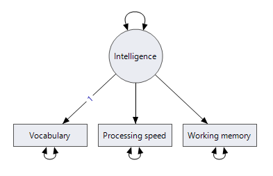
Every full SEM analysis begins with the measurement model, tested through confirmatory factor analysis (CFA). The purpose is to verify that your observed indicators adequately represent the latent constructs you have theorised — before examining any relationships between those constructs. Running a full SEM without validating the measurement model first is the single most common structural error in quantitative dissertations.
What Is CFA?
Confirmatory factor analysis differs from exploratory factor analysis (EFA) in a fundamental way: you specify the factor structure in advance based on theory, then test whether the data confirm it. In lavaan, factor loading relationships are specified with the =~ operator:
model <- '
  # Latent variable definitions (measurement model)
  SelfEfficacy    =~ se1 + se2 + se3 + se4
  ResearchAnxiety =~ ra1 + ra2 + ra3
'
fit <- cfa(model, data = mydata)
summary(fit, fit.measures = TRUE)
Each observed indicator (se1, se2, and so on) loads onto its assigned latent factor. CFA estimates standardised factor loadings (expected between 0.40 and 0.90 for well-constructed scales), intercepts, and residual variances for each indicator. Items with standardised loadings below 0.40 contribute little to defining the construct and may warrant revision or removal before proceeding to the structural model.
Latent Variables: The Core Advantage
Latent variables are inferred from covariance patterns among their indicators. Because the model explicitly estimates measurement error for each observed item, the resulting latent variable is a purer representation of the theoretical construct than a simple composite score or mean. This is the mechanism through which SEM produces less-biased path estimates than multiple regression when your predictors and outcomes involve psychological, social, or educational constructs.
Assessing Convergent and Discriminant Validity
After fitting a CFA model, two forms of construct validity must be established before the structural model is defensible:
| Validity Type | What It Checks | Common Evidence |
|---|---|---|
| Convergent validity | Indicators of the same construct correlate strongly with each other | Average Variance Extracted (AVE) ≥ 0.50; Composite Reliability (CR) ≥ 0.70 |
| Discriminant validity | Different constructs are sufficiently distinct from one another | AVE for each construct exceeds the squared inter-construct correlation (Fornell-Larcker criterion) |
Measurement consistency across raters or instruments is a related concern: the guide to inter-rater reliability covering ICC, Krippendorff’s Alpha, and Bland-Altman provides complementary grounding if your indicators involve coded or observer-rated data rather than self-report scales.
The Structural Model: Path Diagrams and Relationships
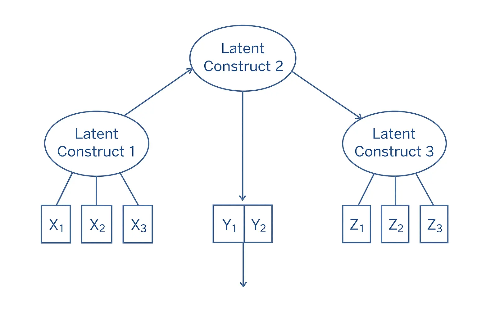
Once the measurement model passes CFA scrutiny, you add the structural model — specifying directional regression paths between the validated latent constructs. This layer is what directly tests your theoretical hypotheses.
In a path diagram, latent variables appear as ovals, observed variables as rectangles, single-headed arrows represent regression paths, and double-headed curved arrows denote correlations. A complete SEM merges both layers in one model specification:
model <- '
  # Measurement model
  SelfEfficacy    =~ se1 + se2 + se3 + se4
  ResearchAnxiety =~ ra1 + ra2 + ra3
  Performance     =~ p1  + p2  + p3

  # Structural model (regression paths among latents)
  Performance     ~ SelfEfficacy + ResearchAnxiety
  ResearchAnxiety ~ SelfEfficacy
'
fit <- sem(model, data = mydata)
summary(fit, fit.measures = TRUE, standardized = TRUE)
Here, SelfEfficacy predicts both ResearchAnxiety and Performance directly, while ResearchAnxiety also predicts Performance. SEM therefore estimates both the direct effect of SelfEfficacy on Performance and the indirect effect routed through ResearchAnxiety — simultaneously, and with measurement-error corrections that simple Baron-Kenny mediation ignores.
The two-step modelling approach (Anderson & Gerbing, 1988) is broadly recommended: establish and confirm the CFA first, then add structural paths. This sequencing prevents structural misspecification from contaminating the measurement parameter estimates that underpin your latent constructs.
How to Assess Model Fit: CFI, RMSEA, and SRMR
Model fit in SEM evaluates how closely the model-implied covariance matrix matches the observed sample covariance matrix. No single index captures all aspects of fit, which is why reporting at least three complementary indices is now standard across journals in psychology, management, and education.
Report SRMR paired with either CFI or RMSEA. Meeting the cutoffs on both provides stronger evidence of fit than any single index in isolation. Reporting all three together gives reviewers the most complete picture of model quality.
| Index | What It Measures | Excellent | Acceptable | Poor |
|---|---|---|---|---|
| CFI | Improvement over a baseline null model (incremental fit) | ≥ 0.95 | 0.90–0.95 | < 0.90 |
| RMSEA | Per-degree-of-freedom misfit, adjusted for model parsimony | ≤ 0.05 | 0.05–0.08 | > 0.10 |
| SRMR | Average standardised residual correlation across all indicator pairs | ≤ 0.06 | 0.06–0.08 | > 0.10 |
The Chi-Square Problem
The model chi-square test remains standard output in every SEM software package, but it is almost never the primary criterion for evaluating fit. Chi-square is extraordinarily sensitive to sample size: with N above roughly 400, even trivially misspecified models tend to produce a statistically significant result. Always report chi-square and its degrees of freedom for transparency, then base substantive fit judgements on CFI, RMSEA, and SRMR.
Critical Caveats on Cutoff Values
The Hu-Bentler cutoffs were derived from simulations using continuous, normally distributed indicators with N ≥ 250 and small-to-moderate models. They are guidelines, not universal laws. Three adjustments are commonly required:
- Small samples (N < 200): RMSEA is artificially inflated at low N. Always report the 90% confidence interval alongside the point estimate so reviewers can assess whether apparent poor fit reflects genuine misspecification or sampling uncertainty.
- Large models (many indicators): CFI naturally drifts downward as model complexity increases. A CFI of 0.92 in a 50-indicator model warrants different interpretation than the same value in a 12-indicator model.
- Categorical or ordinal data: Request scaled versions in lavaan (
cfi.scaled,rmsea.scaled) via the WLSMV estimator. Standard ML-based cutoffs do not apply directly to ordinal data. See the Cornell Statistical Consulting Unit’s SEM fit index reference for a detailed breakdown of index behaviour under varied conditions.
SEM Software: lavaan vs AMOS
Two software ecosystems dominate SEM practice in English-speaking academic research in 2026:
| Feature | lavaan (R) | IBM AMOS |
|---|---|---|
| Cost | Free (open source) | Paid (IBM SPSS add-on) |
| Interface | Script-based syntax in R/RStudio | Drag-and-drop path diagram GUI |
| Reproducibility | Excellent — syntax files are fully reproducible | Limited without scripted output logs |
| Estimators | ML, MLR, MLM, WLSMV, Bayesian | ML, GLS, Bayesian (limited) |
| Missing data | Full-information ML (FIML) natively | FIML available |
| Community & docs | Large, active; peer-reviewed tutorials | Established base in management and business journals |
The UCLA Statistical Consulting Group’s lavaan tutorial is a freely available, peer-vetted resource recommended by many university graduate programmes. AMOS retains a strong foothold in management and organisational behaviour journals where SPSS familiarity predominates, but lavaan’s transparent syntax makes it the stronger choice for dissertations where methodological reproducibility is a committee or examiners’ concern.
The software and statistical approach you choose for SEM is one decision within a broader methodological strategy. If you are still working through the foundational choice between quantitative and qualitative paradigms, the guide to qualitative vs quantitative research design covers those trade-offs systematically.
Four Common SEM Mistakes to Avoid
- Skipping the CFA stage. Running the full SEM without first confirming that the measurement model fits is the most common structural error. A misspecified measurement model corrupts all downstream structural parameter estimates. Validate CFA independently, review loadings, AVE, and CR, then add structural paths.
- Reporting chi-square as the sole fit criterion. Reviewers in 2026 expect a minimum of CFI, RMSEA (with 90% CI), and SRMR. Any submission presenting chi-square alone will draw a request for reanalysis at first revision.
-
Using modification indices without theoretical justification. lavaan’s
modindices()function will always surface parameter tweaks that improve chi-square. Adding them without theoretical warrant inflates fit statistics through capitalisation on chance — equivalent to HARKing (hypothesising after results are known) and reviewable as post-hoc model fishing. - Under-identified models. A model with more free parameters than known data points has negative degrees of freedom and cannot be estimated. The identification rule: df = [p(p+1)/2] − free parameters, where p is the number of observed variables. Models must be over-identified (df > 0) to permit fit evaluation. Check identification before running estimation.
Frequently Asked Questions
What is the difference between SEM and multiple regression?
Multiple regression models one dependent variable at a time using directly observed variables only, and assumes all predictors are measured without error. Structural equation modeling tests an entire network of relationships simultaneously, incorporates latent variables measured indirectly through multiple indicators, and explicitly models measurement error for each indicator. SEM is therefore better suited to testing complex theoretical models in social, educational, and health sciences where key constructs cannot be observed directly.
How many participants do I need for SEM?
The most widely cited working minimum is N ≥ 200, though the adequate sample size depends heavily on model complexity, factor loading magnitudes, and number of indicators per latent variable. Simple models with high loadings (≥ 0.70) can produce stable estimates at smaller samples; complex models with many weakly-loading indicators may require N ≥ 500 or more. The Hu-Bentler fit cutoffs were validated at N ≥ 250 with normally distributed continuous indicators — below this threshold, treat RMSEA in particular as unstable and always report its 90% confidence interval.
Is CFA the same as SEM?
CFA is a subset of SEM. In CFA (the measurement model stage), latent variables are allowed to correlate freely with one another, but no directional regression paths exist between them. Full SEM adds a structural model layer that specifies directional regression paths between latent variables. The distinction matters practically: CFA validates your measurement instruments; the structural model then tests your theoretical hypotheses about how those constructs influence each other.
Which fit indices should I report in my thesis?
Report at minimum: model chi-square with degrees of freedom and p-value (for transparency), CFI (target ≥ 0.95), RMSEA with its 90% confidence interval (target ≤ 0.06 for the point estimate), and SRMR (target ≤ 0.08). If your data are ordinal or categorical, use scaled versions — cfi.scaled and rmsea.scaled — via WLSMV estimation in lavaan. Many journals also request TLI alongside CFI. Reporting chi-square alone is a common cause of revise-and-resubmit feedback in quantitative dissertation examinations.
Can I use SEM to test mediation?
Yes, and SEM is the preferred approach for mediation analysis involving latent variables. Unlike the Baron-Kenny stepwise method or Hayes’s PROCESS macro — which operate on observed variables — SEM models the indirect path through the mediator while simultaneously correcting for measurement error in all constructs. Use bootstrapped confidence intervals for indirect effects (typically 5,000 bootstraps). Bias-corrected bootstrap confidence intervals are more accurate than asymptotic standard errors for indirect effects, particularly in small-to-medium samples.
What is the two-step modelling approach in SEM?
The two-step approach (Anderson & Gerbing, 1988) recommends establishing and confirming the measurement model through CFA first, then adding structural (path) relationships in a second step. This sequencing prevents structural misspecification — wrong or missing paths — from distorting the factor loadings and error variances in your measurement model. Step 1: run CFA and confirm adequate fit plus construct validity (AVE, CR, discriminant validity). Step 2: add structural paths and re-evaluate overall fit. If fit deteriorates substantially at Step 2, the structural hypotheses rather than the measurement model are the most likely source of misfit.
Structure Your SEM Methodology Chapter with Confidence
Articulating your SEM rationale in a methodology chapter — why latent variables over observed-variable regression, which estimator, what fit criteria and why — is as demanding as running the analysis itself. Tesify helps you build a structured, academically coherent methodology chapter that correctly frames your chosen statistical approach, contextualises your fit results against published benchmarks, and connects your methodological decisions to your research questions.
Write your thesis with AI
Structure, draft, cite, and format your thesis faster with Tesify’s AI writing tools, automatic bibliography, and plagiarism checker. Free to start, no credit card required.






Leave a Reply