How to Run an Exploratory Factor Analysis in SPSS (2026): KMO, Bartlett’s, Scree Plot and Rotation

You have 300 completed questionnaires and 24 items, and your supervisor has asked whether the items “hang together” the way your theory says they should. That is an exploratory factor analysis, and in SPSS it is about six clicks and a great deal of judgement. This guide walks the whole procedure end to end: the checks you run before extracting anything, the decision about how many factors to keep, the rotation choice that most students get wrong, and how to write the result up so it survives a methods viva.

Step 1: Check that your data can support a factor analysis at all

Exploratory factor analysis (EFA) looks for a small number of unobserved variables — factors — that explain the pattern of correlations among your measured items. If your items barely correlate with each other, there is no shared variance to explain and no factor structure to find. Three things need to be true before you extract anything.

Your items must be at least ordinal and treated as continuous. Likert-type items are the standard input; the practical convention is that five or more response categories behave well enough for the correlation-based methods SPSS uses. If your scale is still being designed, the item-writing decisions that determine whether EFA will work at all are made much earlier — our guide to designing a Likert scale questionnaire covers that stage.

Your sample must be big enough. The old rules of thumb — 10 participants per item, or a flat minimum of 300 — are crude, and the honest modern answer is that the required N depends on how strong your communalities and loadings are. Fabrigar, Wegener, MacCallum and Strahan (1999, Psychological Methods) made the case that a well-determined structure with high communalities can be recovered with a much smaller sample than the rules of thumb imply, while a weakly determined one will not be recovered even with a large sample. Practically: aim for at least 5–10 cases per item, be uneasy below 150 total, and report your reasoning rather than citing a rule. Formal power planning for other designs is covered in our sample size and power analysis guide.

Your correlation matrix must be factorable. That is what the next step tests.

Step 2: Run the KMO and Bartlett’s tests

In SPSS, go to Analyze → Dimension Reduction → Factor. Move your items into the Variables box. Click Descriptives and tick KMO and Bartlett’s test of sphericity, plus Coefficients and Anti-image under Correlation Matrix. Those four boxes give you everything you need to judge factorability.

The Kaiser–Meyer–Olkin measure of sampling adequacy is a ratio comparing ordinary correlations to partial correlations. When items share a lot of common variance, the partials are small and KMO approaches 1. Kaiser’s own verbal labels for the resulting value are still the ones examiners expect: values in the .90s are excellent, the .80s good, the .70s acceptable, the .60s mediocre, the .50s poor, and anything below .50 unacceptable. A KMO below .50 means you should not proceed without doing something about it.

Bartlett’s test of sphericity asks whether your correlation matrix is significantly different from an identity matrix — one where every item correlates with itself and with nothing else. You want this test to be significant (p < .05). A non-significant Bartlett’s test means your items are essentially unrelated and factor analysis is pointless. Be aware that Bartlett’s is very sensitive to sample size: with 300 cases it is almost always significant, so treat it as a floor condition rather than as evidence of a good structure.

The anti-image correlation matrix is the underused part of this output. Its diagonal holds a KMO value for each individual item. If your overall KMO is acceptable but one item’s individual measure sits below .50, that item is the problem — drop it, re-run, and watch the overall figure rise. Doing this one item at a time is important, because removing an item changes every other item’s value.

Step 3: Choose an extraction method

Click Extraction. SPSS defaults to Principal components, and this is the single most consequential default in the dialog, because principal components analysis is not factor analysis. PCA reduces your items to composite variables that summarise all their variance, including the variance unique to each item and its measurement error. EFA models only the variance items share, which is what you want if you believe an underlying construct causes the item responses.

If your reasoning is “these items are indicators of an underlying trait”, choose Principal axis factoring (robust, makes no distributional assumptions) or Maximum likelihood (allows fit statistics and significance tests, but assumes multivariate normality). Fabrigar and colleagues recommend maximum likelihood when the normality assumption is tenable and principal axis factoring when it is not. Choose principal components only if your goal genuinely is data reduction rather than measuring a construct — and say so explicitly in your methods chapter, because a marker who sees “factor analysis” in your text and “principal components” in your output will ask.

Step 4: Decide how many factors to keep

This is the judgement call that defines your analysis, and SPSS’s default will usually get it wrong.

The default is the Kaiser criterion: retain every factor with an eigenvalue greater than 1 (Kaiser, 1960). An eigenvalue is the amount of variance a factor accounts for expressed in item-units, so the rule says “keep any factor that explains more than a single item would”. It is simple, it is the default, and it is well documented to over-extract — frequently suggesting several more factors than the data really support.

The scree plot (Cattell, 1966) is the visual alternative. Tick Scree plot in the Extraction dialog. It plots eigenvalues in descending order; you look for the “elbow” where the curve flattens into scree, and retain the factors above it. It is genuinely useful and genuinely subjective — two competent readers can see the elbow in different places.

Parallel analysis (Horn, 1965) is the method the methodological literature most consistently recommends. It generates many random datasets with your number of cases and variables, computes their eigenvalues, and tells you to retain only factors whose real eigenvalue exceeds what random noise produced at the same position. It is not on the standard SPSS Extraction dialog, but O’Connor (2000, Behavior Research Methods, Instruments, & Computers) published freely available SPSS syntax macros for parallel analysis and Velicer’s MAP test, and it is built in to the free packages — which is one practical reason to keep one of them installed alongside SPSS, as our comparison of JASP, jamovi, SPSS and R discusses.

The defensible approach for a thesis is to run all three, report where they agree and disagree, and let theory break ties. “Parallel analysis and the scree plot both indicated three factors, while the Kaiser criterion suggested five; the three-factor solution was retained as it was both more parsimonious and consistent with the theorised structure” is a sentence no examiner will argue with.

Step 5: Rotate — and pick the right family

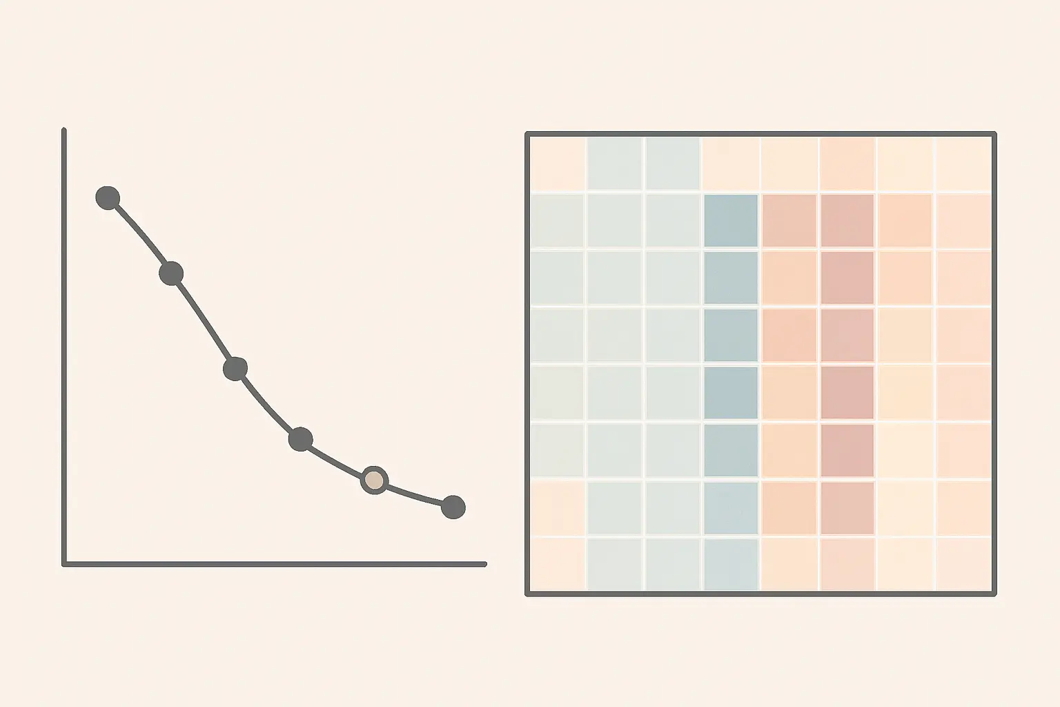
Unrotated factors are mathematically valid and almost never interpretable. Rotation redistributes the loadings to approach “simple structure” — each item loading strongly on one factor and weakly on the rest — without changing how much variance the solution explains overall.

Click Rotation and make the choice that matters: orthogonal or oblique. Orthogonal methods (Varimax is the common one) force the factors to be uncorrelated. Oblique methods (Direct Oblimin, Promax) allow them to correlate. The decision is theoretical, not empirical: do you believe your constructs are related to each other? In social science, subscales of the same instrument almost always are — the facets of job satisfaction are not independent of one another — so oblique rotation is usually the honest default, and Varimax is usually chosen because it is first in the list and produces a tidier-looking table.

There is a self-checking move here. Run an oblique rotation and read the Factor Correlation Matrix that SPSS prints at the bottom of the output. If the inter-factor correlations are all trivially small, an orthogonal rotation was defensible after all and you can report that you checked. If any correlation is substantial, you have empirical grounds for keeping the oblique solution — and Varimax would have suppressed a real relationship.

One output note that confuses people: orthogonal rotation produces a single Rotated Component/Factor Matrix, but oblique rotation produces both a Pattern Matrix and a Structure Matrix. Interpret and report the Pattern Matrix — it holds the unique contribution of each factor to each item, which is what “loading” normally means. The Structure Matrix contains correlations inflated by the factors’ overlap.

Finally, click Options and set Suppress small coefficients to .30 or .40, and tick Sorted by size. This turns a wall of numbers into a readable block structure.

Step 6: Read the solution and deal with bad items

Three things in the output decide whether your solution is any good.

Communalities tell you how much of each item’s variance the retained factors explain. Values below about .30 mean an item has little in common with the rest of the set. Cross-loadings are items loading .32 or higher on two or more factors; they are ambiguous and are the usual candidates for removal. Thin factors — those defined by only one or two items — are unstable and usually should not be retained; three items is the practical minimum for a factor you intend to treat as a subscale.

When you remove an item, remove one, re-run the entire analysis, and re-read the output. Every statistic in it — KMO, eigenvalues, the number of factors suggested, every loading — is conditional on the item set. Iterating item-by-item is slow and it is the only correct way to do it. Record each iteration and why you made it; that log becomes your methods paragraph and is the difference between principled scale refinement and fishing.

Once the structure is stable, compute reliability for each retained factor separately — the factors are your subscales, so a single alpha for the whole instrument is the wrong statistic. Our guide to calculating and reporting Cronbach’s alpha covers the thresholds and their limits.

Step 7: Report it properly

A complete EFA write-up states, in this order: the extraction method and why; the sample size and cases-per-item ratio; the KMO value and the Bartlett’s result; the criteria used to decide the number of factors and what each indicated; the rotation method and the theoretical justification for orthogonal versus oblique; the total variance explained; and a table of the pattern matrix with small loadings suppressed and the suppression threshold stated in the note. If you removed items, say which, in what order, and on what criterion.

Two habits separate a strong write-up from a weak one. Report the decisions, not just the numbers — an examiner can read a loading table, but only you can explain why you kept three factors when Kaiser said five. And keep the italicisation and decimal conventions consistent with the rest of your results, which our guide to writing the results chapter sets out.

One last framing point. EFA is exploratory: it discovers structure. If your aim is to test a structure you already hypothesised, the correct analysis is confirmatory factor analysis, which sits inside the structural equation modelling framework. Running EFA and CFA on the same data and presenting the CFA as confirmation is circular; if you need both, split the sample or collect a second one.

Frequently asked questions

What is a good KMO value for factor analysis?

Above .70 is comfortable, .60 to .70 is mediocre but workable, and below .50 is unacceptable. Check the anti-image correlation matrix diagonal for individual items dragging the overall value down.

What if Bartlett’s test is not significant?

Your items are essentially uncorrelated and there is no shared variance to factor. Do not proceed. Revisit whether the items measure a common construct, and check for data entry problems such as unreversed negatively-worded items.

Should I use Varimax or Direct Oblimin?

Decide on theory: use an oblique rotation such as Direct Oblimin if your factors could plausibly correlate, which for most social science constructs they can. Then read the Factor Correlation Matrix — if all correlations are trivial, you have grounds to report an orthogonal solution instead.

What is the difference between PCA and EFA in SPSS?

Principal components analysis summarises all the variance in your items, including error; exploratory factor analysis models only the variance items share, which is what you want when the items are indicators of a latent construct. SPSS defaults to principal components, so you must change it deliberately.

How many items should load on each factor?

Three is the practical minimum for a factor you plan to treat as a subscale. Two-item factors are unstable across samples, and a single-item factor is not a factor.

Can I remove several bad items at once?

No. Every statistic in the output is conditional on the item set, so removing one item changes the case for removing the others. Remove one, re-run, re-read, and document the sequence.

Do I need to report the unrotated solution?

No. Report the rotated solution you interpreted — the pattern matrix for an oblique rotation. State the rotation method and the suppression threshold in the table note.

Write the analysis up while it is still fresh

The hardest part of an EFA is not the clicking; it is reconstructing three weeks later why you dropped item 14 and kept three factors instead of five. Tesify helps you build the methodology and results chapters as you work, so each decision and its justification lands in the document at the moment you make it — 100% written by you.

Write your thesis with Tesify