
How to Handle Missing Data in Your Dissertation Step by Step (2026): Deletion, Imputation & Reporting
Missing data is one of the most common and least discussed problems in dissertation research. You design a careful survey, collect responses, run your first descriptive statistics — and then notice that 12% of participants skipped the income question, or that three variables in your longitudinal dataset have gaps scattered throughout. How you handle those gaps shapes every finding that follows. Examiners know this, and they expect to see a principled, explicitly justified decision in your methodology chapter, not a silent deletion you hoped they would not notice.
This guide walks you through how to handle missing data in research from first principles: diagnosing which type of missingness you are dealing with, choosing the right technique, implementing it in SPSS or R, and writing it up in APA 7th edition format so your methodology chapter reads as rigorous rather than rushed.
First, classify your missing data as MCAR, MAR, or MNAR using Little’s test and pattern inspection. If MCAR and low rate (<5%), listwise deletion is acceptable. If MAR, use multiple imputation (R mice or SPSS Missing Values module). If MNAR, acknowledge the limitation explicitly and apply sensitivity analysis. Always report the mechanism, rate, and technique used in your results section.
Step 1: Understand the Three Types of Missing Data
The foundational framework for missing data was introduced by Rubin (1976), who distinguished three mechanisms. Every decision you make downstream depends on correctly identifying which applies to your dataset.
Missing Completely at Random (MCAR)
Data are MCAR when the probability of a value being missing has no relationship to any variable in the dataset — observed or unobserved. Think of a survey participant who accidentally skipped a page due to a printing error. The missingness is purely random. MCAR is the least harmful form because it does not introduce systematic bias, though it does reduce statistical power. It is also the easiest to verify.
Missing at Random (MAR)
Data are MAR when the probability of missingness depends on other observed variables in your dataset, but not on the missing values themselves. For example, older participants may be less likely to report their income, but once you account for age, the probability of income being missing does not depend on what that income would have been. MAR is the most common mechanism in social-science dissertations, and it is the assumption that makes multiple imputation valid.
Missing Not at Random (MNAR)
Data are MNAR when the probability of missingness is related to the unobserved value itself. High-earning participants who do not report income because they earn a lot is a classic example. MNAR is the most dangerous form because no standard imputation method can fully correct it — the missingness is informative. It requires a sensitivity analysis and explicit acknowledgement as a study limitation.
Step 2: Diagnose Your Missing Data Mechanism
Before choosing any technique, you must inspect and test your missing data pattern. Two approaches are standard.
Visual Pattern Inspection
In R, the mice package’s md.pattern() function produces a matrix showing which variables are missing and how the patterns cluster. A random scatter across cases and variables is consistent with MCAR. Patterns where the same participants are missing on multiple related variables suggest MAR or MNAR.
Little’s MCAR Test
Little’s test (Little, 1988) produces a chi-square statistic testing the null hypothesis that data are MCAR. Available in SPSS via Analyze → Missing Value Analysis → Little’s MCAR Test, and in R via mcar_test() in the naniar package. A non-significant result (p > .05) supports the MCAR assumption. However, the test has limited power in small samples, so treat it as one piece of evidence rather than a definitive verdict.
Correlating Missingness with Observed Variables
Create a binary indicator (1 = missing, 0 = observed) for each variable with missing values, then correlate those indicators with your other observed variables. Significant correlations suggest the data may be MAR — the missingness is predictable from what you did observe, which is precisely what multiple imputation exploits.
Step 3: Assess the Missing Data Rate
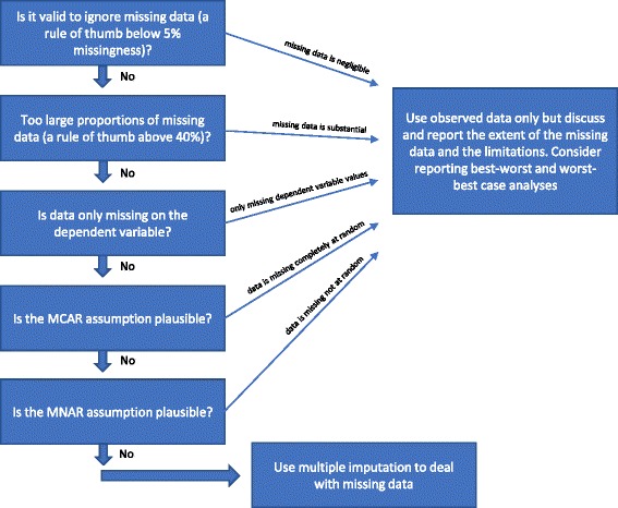
The proportion of missing data matters alongside the mechanism. Common thresholds used in methodological guidance:
| Missing Rate | General Guidance |
|---|---|
| <5% | Listwise deletion is acceptable if data are MCAR; any method works |
| 5–20% | Multiple imputation strongly preferred; document technique thoroughly |
| 20–40% | Multiple imputation required; investigate source of missingness; discuss as limitation |
| >40% | Imputation is unreliable; consider whether the variable is viable; conduct sensitivity analyses |
Report these rates per variable, not just overall. A dataset with 3% missing overall but 35% missing on your primary outcome variable has a fundamentally different problem than one with 3% scattered uniformly across all variables.
Step 4: Choose Your Handling Technique (Decision Table)
Use this decision table to select the appropriate method. The combination of mechanism and rate is what drives the choice.
| Mechanism | Rate | Recommended Technique | Justification |
|---|---|---|---|
| MCAR | <5% | Listwise deletion | No bias introduced; power loss negligible |
| MCAR | 5–20% | Multiple imputation | Preserves power; unbiased under MCAR |
| MAR | Any | Multiple imputation | Uses observed predictors of missingness; valid under MAR |
| MNAR | Any | MI + sensitivity analysis | No unbiased solution; quantify the uncertainty |
| Unknown | <5% | Listwise deletion + MCAR test | Conservative; document uncertainty |
Step 5: Listwise and Pairwise Deletion
Listwise (Complete-Case) Deletion
Listwise deletion removes every case that has a missing value on any variable in the analysis. It is the default in SPSS, R’s lm(), and most statistical software. When data are MCAR and the missing rate is low, this approach is unbiased — effectively equivalent to simple random sampling from a complete dataset. The cost is reduced sample size and statistical power. When data are MAR or the rate is higher, listwise deletion yields biased estimates because the remaining complete cases are no longer representative.
Pairwise Deletion
Pairwise deletion (also called available-case analysis) uses all available data for each specific calculation. When computing a correlation between variables A and B, it uses all cases where both A and B are observed, even if those cases have missing values elsewhere. This retains more data than listwise deletion, but it can produce a non-positive-definite correlation matrix (a matrix that is mathematically impossible), which causes downstream analyses to fail. Use pairwise deletion only for descriptive statistics, never as a primary strategy for handling missing data in regression or structural equation models.
Step 6: Simple Imputation Methods
Simple imputation replaces each missing value with a single estimated value. These methods are fast but have a known statistical flaw: they treat the imputed value as if it were observed, understating uncertainty and producing standard errors that are too small.
Mean Imputation
Replace each missing value with the variable’s observed mean. Mean imputation preserves the variable mean but reduces variance, distorts the distribution, and attenuates correlations with other variables. It is appropriate only for MCAR data with very low missing rates, and even then it should be disclosed as a limitation. Examiners in quantitative-heavy fields will penalise undisclosed mean imputation.
Regression Imputation
Predict missing values from observed variables using a regression model. More accurate than mean imputation because it preserves relationships between variables, but it still understates uncertainty because it treats predicted values as certain. It is a useful intermediate technique when multiple imputation software is unavailable, but it should not be presented as equivalent to multiple imputation.
Last Observation Carried Forward (LOCF)
Common in longitudinal medical studies, LOCF replaces a missing follow-up value with the most recent observed value. It assumes no change over time — an assumption that is often implausible and can seriously bias estimates in either direction. Use LOCF only if it is the standard in your specific field and justify it explicitly.
Step 7: Multiple Imputation — The Gold Standard
Multiple imputation (MI) is the current methodological standard for handling missing data under MAR. Rather than substituting a single value, MI generates m complete datasets (typically m = 5–20), each with slightly different plausible values drawn from the distribution of the missing data given the observed data. You run your analysis on each of the m datasets separately, then combine the results using Rubin’s rules — a pooling procedure that correctly propagates uncertainty from the imputation step into your final estimates.
The reference implementation of MI in R is the mice package (van Buuren & Groothuis-Oudshoorn, 2011), which performs multivariate imputation by chained equations (MICE), also called fully conditional specification. MICE imputes each variable with missing data sequentially using a regression model conditioned on all other variables, cycling through the variables multiple times until the imputed values stabilise. The key advantage is flexibility: it handles continuous, binary, ordinal, and count variables by choosing the appropriate regression model for each.
For best practices in multiple imputation (Woods et al., 2024), include all variables you intend to use in your main analysis in the imputation model, plus any auxiliary variables correlated with missingness. Leaving a variable out of the imputation model but including it in the analysis produces biased estimates.
How Many Imputations?
The guidance from van Buuren’s Flexible Imputation of Missing Data (freely available at stefvanbuuren.name/fimd) is to set m roughly equal to the percentage of incomplete cases. With 20% missing, use at least 20 imputations. The default of 5 in older textbooks is generally too low for modern standards.
Step 8: Running Imputation in SPSS and R
In SPSS
- Go to Analyze → Multiple Imputation → Impute Missing Data Values.
- Move all analysis variables to the “Variables in Imputation Model” box.
- Set the number of imputations (m). Use at least 10 for exploratory work, 20+ for published theses with >15% missing.
- Select imputation method: Fully Conditional Specification (recommended over Monotone for general patterns).
- SPSS creates a new dataset with an Imputation_ index variable (0 = original, 1 to m = imputed datasets).
- Run your analysis as normal — SPSS recognises the imputed structure and automatically pools results using Rubin’s rules for supported procedures (linear regression, logistic regression, mixed models).
- For unsupported procedures, run each imputed dataset separately and pool manually.
In R (mice package)
library(mice)
library(dplyr)

# Step 1: Inspect missing data pattern
md.pattern(your_data)

# Step 2: Run multiple imputation (m = 20 datasets)
imp <- mice(your_data, m = 20, method = "pmm", seed = 123)
# "pmm" = predictive mean matching (good for continuous variables)
# Use "logreg" for binary, "polyreg" for unordered categorical

# Step 3: Fit your model on each imputed dataset
fit <- with(imp, lm(outcome ~ predictor1 + predictor2 + covariate))

# Step 4: Pool results using Rubin's rules
pooled <- pool(fit)
summary(pooled)
Set seed for reproducibility and report it in your methods section. The pooled output gives you the correctly inflated standard errors that reflect imputation uncertainty.
For a broader comparison of statistical tools for your dissertation, see the Tesify guide to data analysis software for thesis research, which covers when SPSS, R, and other tools are the right fit for different methodological designs.
Step 9: How to Report Missing Data in APA 7th Edition
APA 7th edition does not prescribe exact wording, but your missing data report must appear in the Method section (under Data Analysis or Data Screening) and include four elements: the rate, the mechanism, the technique, and the software. Here are worked examples at each level of complexity.
Minimal Report (Listwise Deletion, MCAR, Low Rate)
“Missing data analysis revealed that 3.2% of values were missing across all variables. Little’s (1988) MCAR test was non-significant, χ²(24) = 22.41, p = .55, supporting the assumption of missing completely at random. Cases with missing values were removed via listwise deletion, leaving a final analytic sample of n = 189.”
Standard Report (Multiple Imputation, MAR)
“Missing data ranged from 0% to 18.4% across variables, with the highest missingness on the household income item. Little’s MCAR test was significant, χ²(31) = 48.72, p = .02, indicating the data were not MCAR. Inspection of missingness patterns showed that income missing values were predicted by participant age (r = .23, p = .004), consistent with a missing at random (MAR) mechanism. Accordingly, missing data were handled via multiple imputation using fully conditional specification (van Buuren & Groothuis-Oudshoorn, 2011). Twenty imputed datasets were generated in R (version 4.4.0) using the mice package (version 3.16.0), with all analysis variables included in the imputation model. Results were pooled across imputed datasets using Rubin’s (1987) rules.”
MNAR Sensitivity Report
“There is reason to suspect that non-response on the depression scale is related to symptom severity itself, indicating a potential missing not at random (MNAR) mechanism. As no standard imputation method yields unbiased estimates under MNAR, we conducted our primary analysis using multiple imputation under the MAR assumption and a pattern-mixture sensitivity analysis to assess the robustness of our conclusions to plausible MNAR departures. Results were qualitatively unchanged across scenarios [cite sensitivity analysis table], and the potential bias from MNAR is acknowledged as a study limitation.”
Writing up the analysis section of your dissertation is one area where precision and structure matter enormously. If you are working through your results chapter, the Tesify methodology chapter guide covers how to present your analytical decisions coherently for an examiner audience.
For context on the broader methodological decisions surrounding your analysis — including your research design, sampling approach, and choice between quantitative and qualitative methods — see the step-by-step guide to quantitative research methods.
Tesify helps dissertation students structure and write every chapter — including methodology and results — using AI trained on academic writing conventions. Start writing your dissertation with Tesify →
Frequently Asked Questions
Is listwise deletion ever acceptable in a dissertation?
Yes. Listwise deletion is acceptable when data are MCAR and the missing rate is below approximately 5%. In that scenario, removing incomplete cases is equivalent to simple random sampling and introduces no systematic bias. The cost is reduced sample size and power. You must report the rate, confirm MCAR via Little’s test, and state that listwise deletion was used — do not let the software drop cases silently without disclosing it.
How do I test whether my data are MCAR?
Use Little’s MCAR test, which is available in SPSS (Analyze → Missing Value Analysis) and in R via the naniar package’s mcar_test() function. A non-significant result (p > .05) supports MCAR. You should also visually inspect missing data patterns using md.pattern() in the R mice package or SPSS’s missing value plots, and check whether missingness on any variable correlates significantly with observed variables.
How many imputed datasets should I create?
A widely used rule of thumb is to set the number of imputed datasets (m) roughly equal to the percentage of incomplete cases. If 20% of cases have at least one missing value, create at least 20 imputations. The older default of m = 5 is now considered too low for most dissertation contexts. Higher m reduces Monte Carlo error in your pooled estimates and is computationally inexpensive with modern software.
Can I use mean imputation in my dissertation?
Mean imputation is generally discouraged in contemporary quantitative dissertations because it reduces variance, distorts the correlation structure between variables, and produces standard errors that are too small, leading to inflated Type I error rates. If you have used it for a very small number of missing values under MCAR, disclose it transparently and acknowledge its limitations. For anything above trivial missingness, use multiple imputation instead.
What do I do if my data are MNAR?
No standard method produces unbiased estimates when data are MNAR. The recommended approach for a dissertation is to apply multiple imputation under the MAR assumption as your primary analysis, then conduct a sensitivity analysis (such as a pattern-mixture model or tipping-point analysis) to show how much the MNAR mechanism would have to deviate from your assumption before your conclusions would change. Acknowledge the limitation explicitly in your Discussion section.
Where in my dissertation should I report missing data handling?
Report your missing data analysis and handling strategy in the Data Analysis or Data Screening sub-section of your Method chapter, before your main analysis subsection. In the Results section, briefly re-state the final analytic sample size after any deletions or note that analyses were based on pooled imputed data. If MNAR is a concern, address it again in the Limitations subsection of your Discussion.
Does multiple imputation work with ordinal or binary variables?
Yes. The mice package in R handles different variable types by selecting the appropriate imputation model automatically or allowing you to specify it. Use method = "logreg" for binary variables, "polyreg" for unordered categorical variables, "polr" for ordered categorical (Likert-scale) variables, and "pmm" (predictive mean matching) for continuous variables. SPSS’s Fully Conditional Specification also handles mixed variable types, though with less flexibility in model specification.
What is the difference between multiple imputation and maximum likelihood estimation for missing data?
Full Information Maximum Likelihood (FIML) is an alternative to multiple imputation that estimates model parameters directly from the likelihood of the observed data, without creating completed datasets. Both methods are valid under the MAR assumption and produce similar results in large samples. FIML is built into structural equation modelling software (e.g., lavaan in R, AMOS in SPSS) and is preferred when your entire analysis can be framed as a single model. Multiple imputation is more flexible when you are running multiple different analyses on the same dataset, or when your analysis procedure does not support FIML directly.
For a broader look at how methodological decisions like this fit into the full shape of your analysis chapter, the guide to mixed methods research design and the complete guide to qualitative research methods both discuss how to frame analytical choices in a way that connects cleanly to your research questions.
Write your thesis with AI
Structure, draft, cite, and format your thesis faster with Tesify’s AI writing tools, automatic bibliography, and plagiarism checker. Free to start, no credit card required.






Leave a Reply