

How to Run a Repeated Measures ANOVA in SPSS (2026): Mauchly’s Test, Sphericity and Greenhouse-Geisser
You measured the same people three times — baseline, post-intervention, follow-up — and now SPSS is asking for “within-subject factor names” instead of the grouping variable you expected. Repeated-measures ANOVA is a different dialog, a different data layout and a different assumption from the one-way ANOVA most guides teach, and the assumption is the part that catches people out at submission. This guide runs the whole procedure, including the correction you will almost certainly need to apply.

Step 1: Confirm this is actually your design
A repeated-measures ANOVA is for a within-subjects factor: every participant contributes a score at every level. Three cases qualify. Longitudinal — the same people measured at several time points. Multiple conditions — every participant completes all experimental conditions. Matched pairs or clusters — participants deliberately matched so that each set behaves as one unit.
The reason it needs its own test is that scores from the same person are correlated. Someone who scores highly at baseline tends to score highly at follow-up. A between-subjects ANOVA treats that stable individual difference as unexplained error; a repeated-measures model partitions it out into a separate participant term. The consequence is a smaller error term and substantially more statistical power from the same number of people — which is precisely why within-subject designs are attractive when recruitment is hard. If you are still choosing among the ANOVA family, the between-subjects counterpart is covered in our step-by-step one-way ANOVA guide, which shows what the same output looks like when each participant appears only once.
Two levels only? Use a paired-samples t-test. The repeated-measures ANOVA reduces to exactly that when there are two conditions, and the t-test is the conventional report.
Step 2: Get your data into wide format

This is where most failed attempts begin. SPSS’s repeated-measures procedure requires wide format: one row per participant, and one column per measurement occasion. A participant measured at three time points occupies a single row with three outcome columns — score_t1, score_t2, score_t3.
Data exported from survey platforms or collected on paper often arrives in long format instead: one row per observation, so each participant occupies three rows with a “time” column marking which is which. Feed that to the one-way ANOVA dialog and SPSS will happily run — treating your 30 participants as 90 independent people. The test completes, the output looks normal, and every number in it is wrong. Restructure first with Data → Restructure → Restructure selected cases into variables.
Handle missing data before you start, too. Repeated-measures ANOVA uses listwise deletion: a participant missing any single time point is dropped from the analysis entirely. In a three-wave study with ordinary attrition this can silently remove a large share of your sample, so check the “N” reported in the output against the number you recruited, and if the gap is large, our guide to handling missing data covers the alternatives.
Step 3: Run the analysis
Go to Analyze → General Linear Model → Repeated Measures. Unlike other dialogs, this one opens with a definition box rather than a variable list.
- Name the within-subject factor. Replace “factor1” with something meaningful —
time— and enter the Number of Levels (3 for three time points). Click Add, then Define. - Assign your variables in order. The next box lists numbered slots. Put
score_t1in slot 1,score_t2in 2,score_t3in 3. The order is the factor’s order, and getting it wrong scrambles every contrast and plot without producing any error message. - Plots. Move
timeto the Horizontal Axis, click Add. A profile plot of the marginal means is the single most useful thing in the output. - Options (or EM Means). Move
timeinto the estimated marginal means box, tick Compare main effects, and set the confidence interval adjustment to Bonferroni. Tick Descriptive statistics and Estimates of effect size.
Note that the pairwise comparisons for a within-subjects factor live under Options/EM Means, not under the Post Hoc button — that button only serves between-subjects factors and will appear greyed out or unhelpful. Students frequently conclude the analysis “will not do post-hocs”. It will; they are somewhere else.
Step 4: Read Mauchly’s test of sphericity
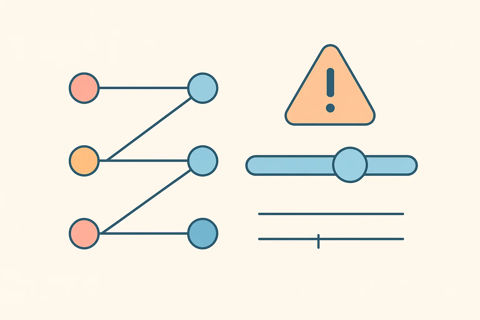
Sphericity is the assumption that replaces homogeneity of variance in within-subjects designs. It requires that the variances of the differences between every pair of conditions be roughly equal: the spread of (t1 − t2) scores, of (t1 − t3) scores and of (t2 − t3) scores should be similar. It is a real risk in longitudinal data, where measurements taken close together are usually more alike than measurements far apart.
Violating it inflates the Type I error rate — your F becomes too liberal and you find effects that are not there. SPSS tests it automatically with Mauchly’s test of sphericity, and here the logic runs the opposite way to most tests you have used:
- Mauchly’s p > .05 — sphericity is not violated. Read the row labelled Sphericity Assumed.
- Mauchly’s p < .05 — sphericity is violated. Do not read that row; use a correction.
Sphericity cannot be violated with only two levels, so with a two-level factor SPSS reports Mauchly’s as a blank or a perfect 1.000. That is not an error.
Step 5: Apply the right correction
You do not abandon the analysis when sphericity fails. The corrections adjust the degrees of freedom downward by a factor called epsilon (ε), making the test more conservative. SPSS prints all of them in the “Tests of Within-Subjects Effects” table, and you simply read a different row.
| Situation | Row to read | Why |
|---|---|---|
| Mauchly’s non-significant | Sphericity Assumed | No adjustment needed |
| Violated, Greenhouse-Geisser ε < .75 | Greenhouse-Geisser | The conservative correction; appropriate for a substantial departure |
| Violated, Greenhouse-Geisser ε > .75 | Huynh-Feldt | Greenhouse-Geisser over-corrects and costs power when the departure is mild |
| Unsure, or reporting conservatively | Greenhouse-Geisser | The safe default; never criticised as too liberal |
The practical consequence is visible in the output: corrected degrees of freedom stop being whole numbers. Instead of F(2, 58) you report something like F(1.62, 46.98). Fractional degrees of freedom are not a mistake — they are the evidence that you applied the correction, and an examiner looks for them.
The fourth row, Lower-bound, is the maximum possible correction and is far too conservative for routine use. Ignore it.
Step 6: Follow up a significant effect
A significant main effect of time tells you the means differ somewhere across the three occasions, not where. The pairwise comparisons you requested in Options answer that, and the Bonferroni adjustment you set controls the family-wise error rate across the three comparisons.
Read them alongside the profile plot: the plot shows the shape of the change, the comparisons tell you which specific gaps are reliable. A pattern where scores rise sharply from baseline to post-intervention and then hold steady at follow-up is a different finding from one where they rise steadily throughout, and the pairwise table is what distinguishes them.
Report effect size as partial eta squared (ηp2), which SPSS gives you if you ticked the box. Be careful describing it: partial eta squared is the proportion of variance explained after removing variance attributable to other terms in the model, so it is not comparable to an r² and values from repeated-measures designs are typically larger than their between-subjects equivalents. Say which one you are reporting. Our guide to effect sizes and confidence intervals covers the interpretation.
Step 7: Write it up
A complete report contains, in order: the design and the within-subject factor with its levels; the outcome of Mauchly’s test; the correction applied and why; the F statistic with its (possibly fractional) degrees of freedom, the p value and partial eta squared; the pairwise comparisons with their adjustment; and descriptive statistics for each occasion.
The sentence pattern examiners expect runs: “Mauchly’s test indicated that the assumption of sphericity had been violated, χ²(2) = 8.41, p = .015; degrees of freedom were therefore corrected using Greenhouse-Geisser estimates of sphericity (ε = .71). There was a significant effect of time on the outcome, F(1.42, 41.18) = 12.63, p < .001, ηp2 = .30.” Two sentences carry the assumption check, the correction, the test and the effect size — and the fractional degrees of freedom prove the correction was real. For the conventions governing the rest of the chapter, see our guide to writing the results chapter.
What to do when the assumptions fail badly
Sphericity has a correction, so it is rarely fatal. Two other problems have no equivalent fix.
If your residuals are severely non-normal and your sample is small, the rank-based alternative for a one-factor within-subjects design is the Friedman test, followed by Wilcoxon signed-rank tests with a Bonferroni adjustment. You lose some power and you can no longer speak about means, but the inference is sound; our overview of non-parametric tests covers the trade-off.
If attrition has removed a substantial part of your sample through listwise deletion, no correction inside this procedure helps, because the missing data problem happened before the test ran. A linear mixed model handles incomplete cases without discarding participants and is the standard modern alternative for longitudinal data — worth raising with your supervisor before you settle for a shrunken N.
Frequently asked questions
What does it mean if Mauchly’s test is significant?
Sphericity is violated: the variances of the differences between pairs of conditions are unequal. Apply a correction — Greenhouse-Geisser or Huynh-Feldt — and read that row of the within-subjects effects table rather than the “Sphericity Assumed” row.
Should I use Greenhouse-Geisser or Huynh-Feldt?
Use Greenhouse-Geisser when its epsilon is below .75, Huynh-Feldt when epsilon exceeds .75 because Greenhouse-Geisser then over-corrects. Greenhouse-Geisser alone is a defensible conservative default.
Why are my degrees of freedom decimals?
Because a sphericity correction multiplied them by epsilon. Fractional degrees of freedom are correct and expected — report them as SPSS gives them, to two decimal places.
Why is the Post Hoc button not working for my within-subjects factor?
That button handles between-subjects factors only. For a repeated-measures factor, request pairwise comparisons in Options or EM Means by ticking “Compare main effects” and choosing Bonferroni.
Does my data need to be in long or wide format?
Wide: one row per participant, one column per measurement occasion. Long-format data run through this procedure treats each observation as a separate person and invalidates the analysis.
What if a participant missed one time point?
They are excluded entirely by listwise deletion. Compare the N in your output with the number recruited; if the loss is substantial, consider a linear mixed model, which retains participants with incomplete data.
Can I run a repeated measures ANOVA with two conditions?
You can, but it is identical to a paired-samples t-test, which is the conventional way to report a two-level within-subjects comparison. Sphericity does not apply with only two levels.
Record the correction while you are looking at it
The detail most often missing from a submitted methods chapter is the sphericity decision — which correction was applied, on what epsilon, and why. Tesify helps you draft the methodology and results sections as you run the analysis, so the justification is written while the output is still on screen — 100% written by you.
Write your thesis with AI
Structure, draft, cite, and format your thesis faster with Tesify’s AI writing tools, automatic bibliography, and plagiarism checker. Free to start, no credit card required.






Leave a Reply