
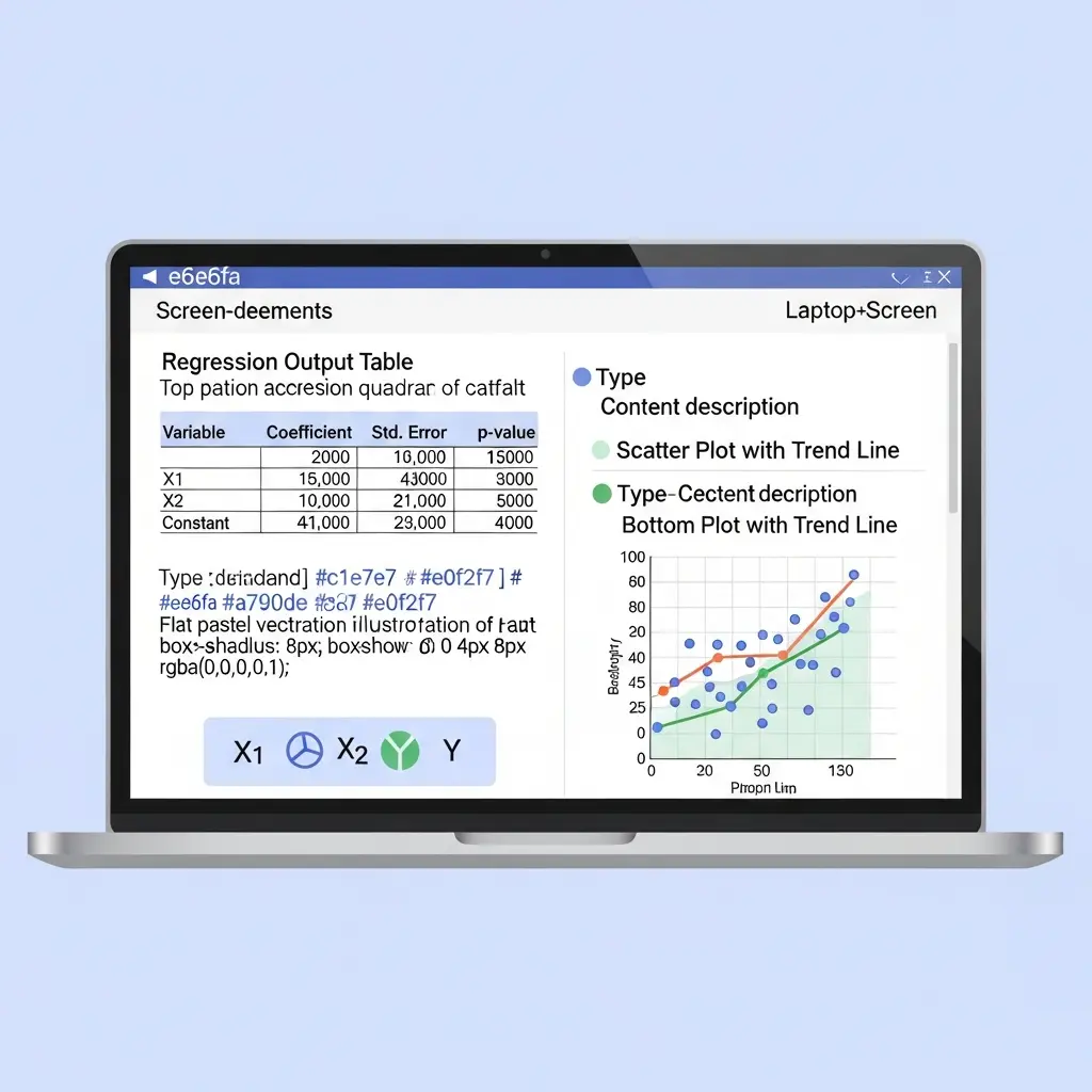
How to Run a Multiple Regression in SPSS and Report It in APA (2026)
Multiple regression is one of the most widely used statistical techniques in social science, psychology, education, public health, and business research. If you need to know how to run multiple regression in SPSS, you have arrived at the right place. This guide walks you through every stage — from setting up your data to navigating SPSS menus, checking the five core assumptions, interpreting all sections of the output, and writing a publication-ready APA 7 results section with a correctly formatted regression table.
Whether you are completing an undergraduate dissertation, a master’s thesis, or a PhD chapter, this tutorial gives you the exact steps and the exact language your markers and examiners expect to see. Unlike generic statistics textbooks, every instruction below maps directly to what you see on screen in IBM SPSS Statistics versions 26–29.
1. What is multiple regression — and when should you use it?
Multiple linear regression estimates the relationship between one continuous outcome variable (also called the dependent variable or criterion) and two or more predictor variables (independent variables). The model takes the form:
Y = b0 + b1X1 + b2X2 + … + bkXk + ε
Each b coefficient tells you how much the outcome changes for a one-unit increase in that predictor, holding all other predictors constant. This controlling-for-others property is what makes multiple regression so powerful for observational research: it lets you isolate the contribution of each variable.
Use multiple regression when:
- Your outcome variable is continuous (e.g., exam score, job satisfaction rating, systolic blood pressure).
- You have two or more predictors whose independent effects you want to examine simultaneously.
- You want to statistically control for confounders (e.g., controlling for age and gender while estimating the effect of study hours on grade).
- You want to build a prediction model and quantify how much variance in the outcome your predictors collectively explain.
If you have already established scale reliability for your measures using SPSS, see our companion guide on how to calculate Cronbach’s alpha in SPSS before running your regression. Scales with poor reliability attenuate your regression coefficients. For understanding how to design the questionnaire instruments whose scores you will enter as predictors, see our guide on how to design a Likert scale questionnaire for your thesis.
2. Before you start: data requirements
Running the analysis before your data meet minimum requirements is the most common source of problems in student dissertations. Work through this checklist first.
| Requirement | Minimum standard | Where to check in SPSS |
|---|---|---|
| Level of measurement | Outcome = continuous (interval/ratio); predictors = continuous or binary | Variable View → Measure column |
| Sample size | ≥10–20 cases per predictor; ≥50 cases minimum | Analyze → Descriptive Statistics → Frequencies (check N) |
| Missing data | Inspect and address before running; SPSS uses listwise deletion by default | Analyze → Descriptive Statistics → Descriptives |
| Outliers | Check Cook’s Distance and standardised residuals (|z| > 3.3) | Save menu in Linear Regression → Cook’s Distance, Standardized residuals |
| Categorical predictors | Must be dummy-coded (0/1) before entry | Transform → Recode into Different Variables |
3. Step-by-step: running multiple regression in SPSS
These steps apply to IBM SPSS Statistics versions 26 through 29. The menu layout is identical across all recent versions. The dialog box carries the title “Linear Regression” — this is correct even when you have multiple predictors.
Step 1: Open the Linear Regression dialog
From the SPSS menu bar, click Analyze → Regression → Linear. The Linear Regression dialog box opens.
Step 2: Assign your variables
- From the variable list on the left, click your outcome variable and move it into the Dependent box using the arrow button.
- Click each predictor variable in turn and move them all into the Independent(s) box (labelled “Block 1 of 1”).
- In the Method dropdown, select Enter. This forces all predictors into the model simultaneously — the appropriate choice for a standard (forced-entry) multiple regression. Use Stepwise only if your research design explicitly calls for exploratory predictor selection, and be aware of its limitations for confirmatory inference.
Step 3: Request statistics
Click the Statistics button. In the dialog that opens, tick the following boxes:
- Estimates — regression coefficients (B and β) with standard errors and t-tests
- Confidence intervals — 95% CIs for each B (required for APA 7)
- Model fit — R and R²
- R squared change — useful if you are entering predictors in hierarchical blocks
- Descriptives — means, SDs, and a correlation matrix (useful for reporting and checking pairwise correlations)
- Collinearity diagnostics — produces VIF and Tolerance values for checking multicollinearity
Click Continue.
Step 4: Request residual plots
Click the Plots button. In the Scatter section:
- Move ZRESID (standardised residuals) to the Y box.
- Move ZPRED (standardised predicted values) to the X box.
- Tick Histogram and Normal probability plot in the Standardized Residual Plots section.
Click Continue.
Step 5: Save diagnostic variables (optional but recommended)
Click the Save button. Tick Cook’s Distance and Standardized (residuals). These are saved as new variables in your dataset and help you identify influential cases and outliers. Click Continue.
Step 6: Run the analysis
Click OK. SPSS runs the regression and opens the output in the Viewer. You will see several tables: Descriptive Statistics, Correlations, Variables Entered, Model Summary, ANOVA, and Coefficients.
4. Checking the five assumptions
Multiple regression rests on five assumptions. Violations do not automatically invalidate your analysis, but they must be examined and discussed in your dissertation’s limitations section. For guidance on writing that section, see our article on how to write a research limitations section in your thesis. To understand how assumption violations relate to the broader concept of research validity, see our guide on construct, internal, and external validity in research design.
Assumption 1: Linearity
The relationship between each predictor and the outcome should be approximately linear. How to check: Examine the ZRESID vs ZPRED scatterplot. The residuals should show no systematic curved pattern — just a roughly rectangular cloud centred on zero. If you see a U-shape or inverted U-shape, linearity may be violated and you should consider adding a squared term or a transformation.
Assumption 2: Independence of errors
Residuals should be independent of each other — no systematic pattern over time or sequence. How to check: Examine the Durbin-Watson statistic in the Model Summary table. Values between 1.5 and 2.5 are generally acceptable; values near 2.0 indicate little autocorrelation. This assumption is most relevant when your data have a time-series or nested structure.
Assumption 3: Homoscedasticity
The variance of the residuals should be constant across all levels of the predicted values. How to check: Look at the ZRESID vs ZPRED scatterplot. Points should be roughly equally spread above and below zero across the full range of the X axis — a “shotgun blast” appearance. A funnel shape (residuals widening as predicted values increase) indicates heteroscedasticity, which inflates standard errors and can make your p-values unreliable.
Assumption 4: Normality of residuals
The residuals should be approximately normally distributed. How to check: Examine the Normal P-P Plot. The data points should track closely along the diagonal reference line. The histogram of standardised residuals should approximate a bell curve. Small deviations are common and acceptable, especially with samples above 100 — regression is fairly robust to mild non-normality when N is large.
Assumption 5: No multicollinearity
Predictor variables should not be too highly correlated with each other. How to check: Look at the VIF (Variance Inflation Factor) and Tolerance columns in the Coefficients table.
| VIF value | Tolerance | Interpretation |
|---|---|---|
| <5 | >0.20 | No multicollinearity concern |
| 5–10 | 0.10–0.20 | Moderate — note but proceed with caution |
| >10 | <0.10 | Serious — remove or combine the redundant predictor |
The VIF thresholds above follow widely cited guidance from Statistics Solutions and are consistent with IBM SPSS documentation. Some researchers use a more conservative threshold of VIF < 5; others accept up to 10. The key point is to report what you found and discuss any values that approach or exceed your chosen threshold.
5. Interpreting SPSS multiple regression output
SPSS produces four key tables. Here is what to read in each one.
Model Summary table
This table reports R, R², and Adjusted R².
- R: the multiple correlation coefficient — the correlation between the observed outcome values and the model’s predicted values. Ranges from 0 to 1.
- R²: the coefficient of determination — the proportion of variance in the outcome explained by all predictors combined. R² = .35 means the predictors collectively account for 35% of the variance.
- Adjusted R²: R² penalised for the number of predictors and the sample size. This is the value to report in APA write-ups with multiple predictors, because it gives a more honest estimate of how well the model would generalise to new data. Always report adjusted R² alongside R².
- Durbin-Watson: check this for independence of errors (see Assumption 2 above).
ANOVA table
This tests whether the overall regression model explains a statistically significant amount of variance in the outcome.
- F-statistic: the ratio of variance explained by the model to unexplained variance.
- df: degrees of freedom — two values are needed. Regression df = number of predictors (k); Residual df = N − k − 1.
- Sig.: the p-value for the F-test. If p < .05, the model as a whole predicts the outcome significantly better than chance.
Coefficients table
This is the most important table for interpreting individual predictors.
| Column | What it means | Use for APA? |
|---|---|---|
| B (Unstandardised) | Predicted change in outcome per 1-unit increase in predictor; in original measurement units | Yes — report with 95% CI |
| SE (Std. Error of B) | Precision of the B estimate | Optional (replaced by CI in APA 7) |
| β (Beta, Standardised) | B expressed in standard deviation units — allows comparison of relative predictor strength within the model | Yes — report alongside B |
| t | t-statistic testing whether B differs significantly from zero | Yes |
| Sig. | Two-tailed p-value for t-test; report to 3 decimal places; use exact value, not just “p < .05” | Yes |
| VIF | Variance Inflation Factor — multicollinearity indicator | Report in text (usually not in main table) |
6. Reporting multiple regression results in APA 7
APA 7th edition (American Psychological Association, 2020) introduced stronger requirements for statistical reporting, particularly the inclusion of confidence intervals. The format below follows current APA 7 guidelines as described in the Publication Manual of the American Psychological Association (7th ed.) and is consistent with guidance from Stats for Scholars’ regression reporting guide.
Structure of an APA regression results paragraph
A complete APA 7 regression write-up has three elements:
- State the analysis and overall model fit — identify the test, report R², adjusted R², F, df, and p.
- Report each predictor — report B with 95% CI, β, t, and p for each variable.
- Refer to the table — direct the reader to your formatted regression table for the full coefficient information.
Illustrative example write-up
The following is an illustrative example. The dataset, variable names, and numerical values are fictional and intended purely to demonstrate correct APA 7 reporting format. Do not treat these figures as real research findings.
A multiple linear regression was conducted to examine whether study hours per week (X1), self-efficacy score (X2), and prior grade point average (X3) predicted final examination score. Preliminary analyses confirmed that the assumptions of linearity, independence of errors (Durbin-Watson = 1.93), homoscedasticity, normality of residuals, and absence of multicollinearity (all VIFs < 3.2) were satisfied.
The overall regression model was statistically significant, R² = .42, adjusted R² = .40, F(3, 146) = 35.47, p < .001, indicating that the three predictors collectively accounted for 42% of the variance in examination scores. Study hours (b = 3.84, 95% CI [2.61, 5.07], β = .41, t(146) = 6.17, p < .001) and prior GPA (b = 8.25, 95% CI [5.93, 10.57], β = .38, t(146) = 7.01, p < .001) were significant positive predictors of examination score. Self-efficacy was not a statistically significant predictor (b = 0.72, 95% CI [−0.14, 1.58], β = .09, t(146) = 1.65, p = .101). Full coefficient information is presented in Table 1.
Key APA 7 formatting rules for regression
- Use italics for all statistical symbols: R², F, p, b, β, t, N.
- Report exact p-values to three decimal places (e.g., p = .034). Use p < .001 only when the value rounds below .001.
- Omit the leading zero before decimals for values bounded between −1 and 1 (e.g., R² = .42, not 0.42).
- Always include both df values with F: F(df_regression, df_residual).
- Report 95% CIs for every B coefficient: [lower bound, upper bound].
- Report both R² and adjusted R² for multiple regression models.
When you format the data table, follow APA table formatting rules precisely. See our step-by-step guide on how to format APA tables and figures for correct rules on borders, alignment, and table notes.
7. Example APA regression table
The table below illustrates the correct APA 7 format for a multiple regression results table. Values are fictional (illustrative example only).
Table 1
Multiple Regression Results Predicting Examination Score (N = 150)
| Variable | b | 95% CI | β | t | p |
|---|---|---|---|---|---|
| Constant | 12.40 | [7.82, 16.98] | 5.34 | <.001 | |
| Study hours per week | 3.84 | [2.61, 5.07] | .41 | 6.17 | <.001 |
| Self-efficacy scale | 0.72 | [−0.14, 1.58] | .09 | 1.65 | .101 |
| Prior GPA | 8.25 | [5.93, 10.57] | .38 | 7.01 | <.001 |
Note. CI = confidence interval. R² = .42; adjusted R² = .40. F(3, 146) = 35.47, p < .001. All values are illustrative; this is not a real dataset.
Notice the APA table conventions applied here: double top border, single line after the header, double bottom border, no vertical lines, table number in plain text above, italicised table title below the number, and a “Note.” at the bottom for abbreviations and model-level statistics.
8. Common mistakes to avoid
Mistake 1: Reporting only p-values and ignoring effect size
Statistical significance tells you whether an effect is likely real, not whether it is practically meaningful. Always report R², adjusted R², and standardised β values. If a predictor is significant but β = .06, that effect may be trivially small in practical terms.
Mistake 2: Using stepwise regression for confirmatory research
Stepwise methods (Forward, Backward, Stepwise) use p-values to decide which predictors to enter or remove. They capitalise on chance in your specific sample and often produce models that replicate poorly. Use Enter (forced entry) for testing theoretically motivated hypotheses. If your research question is genuinely exploratory, note this limitation explicitly in your methodology chapter — our guide on how to write a dissertation methodology chapter step by step covers this distinction in detail.
Mistake 3: Omitting assumption checks from the write-up
Many dissertations run the regression but make no mention of assumptions. Examiners expect you to confirm that assumptions were checked. Even a single sentence per assumption is sufficient: “The assumption of homoscedasticity was assessed by examining the ZRESID vs ZPRED scatterplot; no heteroscedastic pattern was observed.”
Mistake 4: Treating Adjusted R² as a percentage without context
Adjusted R² = .38 means the model accounts for approximately 38% of outcome variance. What counts as a “good” R² is highly discipline-dependent — social science models often explain 20–40% of variance, while clinical or epidemiological models may explain far less. Always contextualise your R² against similar studies in your field.
Mistake 5: Forgetting to dummy-code categorical predictors
If you have a categorical variable with three or more categories (e.g., nationality: British, American, Australian), you must create dummy variables (k−1 binary variables) before entering them into the regression. Entering a categorical variable coded 1, 2, 3 as if it were continuous will produce meaningless coefficients.
Mistake 6: Not saving or reporting your SPSS syntax
Reproducibility is increasingly expected at all levels of academic work. Use Paste instead of OK to save your syntax to a Syntax Editor file before running. This gives you a complete, replicable record of every analysis decision.
Mistake 7: Choosing a statistical package without considering alternatives
If you are deciding between SPSS, JASP, jamovi, and R, our comparison of JASP vs jamovi vs SPSS vs R for thesis statistics in 2026 covers the key differences in interface, reproducibility, and output format — so you can confirm SPSS is the right tool before you commit to it. Korean researchers can find a structured introduction in this Korean-language guide to quantitative research methods.
Frequently asked questions
What is the difference between multiple regression and simple regression in SPSS?
Simple linear regression examines the relationship between one predictor and one outcome variable. Multiple regression includes two or more predictors simultaneously, allowing each predictor’s unique contribution to be estimated while statistically controlling for the others. In SPSS, both use the same Analyze → Regression → Linear menu — you simply add more variables to the Independent(s) box for multiple regression.
What VIF value indicates a multicollinearity problem in SPSS?
A VIF above 10 (or Tolerance below 0.1) is the conventional threshold for serious multicollinearity. Values between 5 and 10 warrant caution and should be discussed. If VIF exceeds 10 for any predictor, consider removing the redundant variable, combining correlated predictors into a composite, or using ridge regression as an alternative. Always report VIF values in your dissertation’s assumption-checking section.
How do I report a non-significant regression model in APA?
Report exactly as you would a significant model — include R², adjusted R², F, df, and p. For example: “The regression model did not significantly predict the outcome, R² = .04, adjusted R² = .01, F(2, 87) = 1.89, p = .157.” Do not omit or minimise non-significant results. A null result is a legitimate finding and should be discussed in terms of effect size and potential reasons (e.g., underpowered sample, inappropriate predictor selection).
Should I report B or beta (β) in my APA regression table?
APA 7 recommends reporting both. The unstandardised B (with its 95% CI) lets readers interpret the effect in the original measurement units and is essential for practical significance. The standardised β allows cross-predictor comparison within the same model. Include both columns in your regression table.
How many participants do I need for multiple regression in SPSS?
A widely cited rule of thumb is 10–20 observations per predictor. For a formal power analysis, use G*Power (free software): for a medium effect size (f² = .15), three predictors, α = .05, and power = .80, you need approximately 77 participants. Consult your supervisor about the expected effect size in your specific field before finalising your sample size target. Document your a priori power calculation in the methodology chapter.
Can I run multiple regression in SPSS with categorical predictors?
Yes, but categorical variables with more than two categories must first be dummy-coded. For a variable with three categories, create two dummy variables (one category serves as the reference group). Binary variables coded 0/1 can be entered directly. In SPSS, use Transform → Recode into Different Variables to create your dummy variables before running the regression. Name your reference category clearly and state it in your results write-up.
Where to go next
Running multiple regression in SPSS is a three-stage skill: setting up the analysis correctly, verifying that assumptions hold, and translating output into clear academic prose. This guide has walked you through every stage with the specific menu paths, assumption diagnostics, and APA 7 conventions you need. Korean-speaking students new to the software will find this Korean-language guide to how to use SPSS a helpful starting point.
If your data are qualitative rather than quantitative, our guide on how to run thematic analysis in NVivo step by step covers the equivalent workflow for qualitative data. For scale development and reliability analysis that typically precedes regression, revisit our guide on calculating Cronbach’s alpha in SPSS. To understand what regression results tell you about how well your study measures what it sets out to measure, see our guide on interpreting confidence intervals correctly.
For the writing itself — drafting your methodology section, results chapter, and keeping your APA references accurate throughout — Tesify provides AI-assisted thesis writing with built-in academic structure and automatic referencing via Auto Bibliography, so you can focus your energy on your analysis rather than formatting compliance.
Write your thesis with AI
Structure, draft, cite, and format your thesis faster with Tesify’s AI writing tools, automatic bibliography, and plagiarism checker. Free to start, no credit card required.




Leave a Reply